7. Deep Learning (Neural Networks)

7.1. What is neural network?

A neural network, within the realm of artificial intelligence (AI), imparts to computers the ability to process data in a manner inspired by the human brain. Operating as a form of deep learning, this method employs interconnected nodes or neurons arranged in layered structures reminiscent of the human brain. This establishes an adaptive system wherein computers learn from errors and consistently enhance their performance. Consequently, artificial neural networks strive to address intricate problems, enabling computers to make intelligent decisions with minimal human intervention. This capability arises from their capacity to grasp and model the intricate, nonlinear relationships between input and output data.

Neural networks find application in various industries, including but not limited to:

\(\bullet\) Medical diagnosis through the classification of medical images.

\(\bullet\) Targeted marketing via social network filtering and analysis of behavioral data.

\(\bullet\) Financial predictions through the analysis of historical data related to financial instruments.

\(\bullet\) Forecasting electrical load and energy demand.

\(\bullet\) Process and quality control.

\(\bullet\) Identification of chemical compounds.

The design of neural network architecture draws inspiration from the human brain. In the human brain, neurons, the fundamental units, create an intricate, highly interconnected network, transmitting electrical signals to facilitate information processing. Similarly, artificial neural networks are comprised of artificial neurons, represented as software modules or nodes, working collaboratively to tackle problem-solving tasks. These artificial neurons operate within software programs or algorithms that leverage computing systems for mathematical calculations.

7.2. Neural networks architecture

The structure of a basic neural network involves three interconnected layers:

\(\bullet\) Input Layer:

External information enters the artificial neural network through the input layer. Input nodes within this layer process, analyze, or categorize the data before passing it on to the next layer.

\(\bullet\) Hidden Layer:

Hidden layers receive input from the input layer or other hidden layers. Neural networks can feature multiple hidden layers, with each layer analyzing output from the preceding layer, further processing it, and transmitting it to the subsequent layer.

\(\bullet\) Output Layer:

The output layer presents the final result of the artificial neural network’s data processing. It may consist of a single node or multiple nodes, depending on the task. For instance, in a binary classification scenario (yes/no), the output layer may have one node yielding a result of 1 or 0. In contrast, a multi-class classification problem might involve an output layer with more than one node.

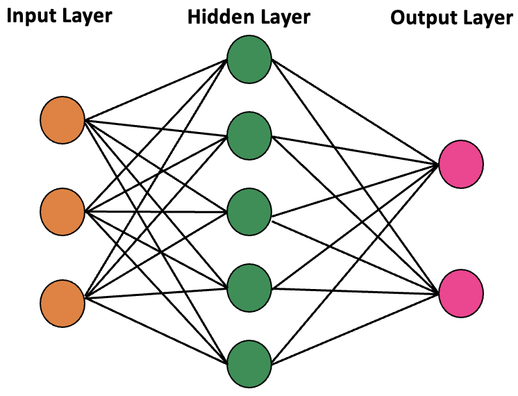
Figure. 20 General structure of a neural network

Artificial neural networks can be classified based on the flow of data from the input node to the output node. Here are some examples:

1. Feedforward Neural Networks:

\(\bullet\) Data is processed in a unidirectional manner, moving from the input node to the output node.

\(\bullet\) Each node in one layer is connected to every node in the subsequent layer.

\(\bullet\) Feedforward networks utilize a feedback process to iteratively enhance predictions over time.

2. Backpropagation Algorithm:

Neural networks achieve continuous learning through corrective feedback loops, refining their predictive analytics. Conceptually, data traverses multiple paths from the input node to the output node within the neural network. A feedback loop is employed in the backpropagation algorithm, following these steps:

\(\bullet\) Each node generates a prediction for the next node in the path.

\(\bullet\) The correctness of the prediction is assessed, with higher weight values assigned to paths associated with correct predictions and lower weight values to paths leading to incorrect predictions.

\(\bullet\) For the next data point, nodes make new predictions using the weighted paths and repeat the process outlined in Step 1.

In the next section, the mathematical framework of a simple neural network will be explained in detail. We consider a neural network with 4 input data. Each data has 2 dimensions. We also assume, there is 1 hidden layer including 3 neurons. For every single input data, we have 1 output which is either 0 or 1 (These are actual values).

First we need to go through the Feedforward process and then implement Backpropagation.

7.3. Feedforward procedure

The structure of our neural network and several steps involved in Feedforward process are shown in this figure:

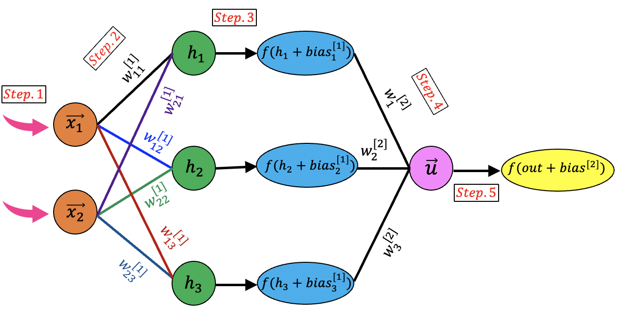
Figure. 21 Feedforward steps in the neural network

\(\textbf {Step.1}\)

First we need to make a matrix including the input data. In general, this is a \([d \times n]\) matrix where \(d\) and \(n\) correspond to the dimensions (i.e., 2) and number of input data (i.e., 4) respectively. This is the very first step of Feedforward implementation in our neural network. According to the fact that we have 4 input data, the \(\boldsymbol{X}\) matrix is formed as following:

(119)\[\begin{split} \boldsymbol{X} = \begin{bmatrix} x_{11} & x_{12} & x_{13} & x_{14} \\ x_{21} & x_{22} & x_{23} & x_{24} \\ \end{bmatrix}\end{split}\]

\(\textbf {Step.2}\)

The values of the \(\boldsymbol{W^{[1]}}\) matrix are initially determined by generating random numbers between 0 and 1 for each element. In the second step, we need to make a matrix including the weights values(\(\boldsymbol{W^{[1]}}\)). This is a \([r \times d]\) matrix where \(r\) is the number of the neurons in the hidden layer (i.e., 3):

(120)\[\begin{split} \boldsymbol{W^{[1]}} = \begin{bmatrix} {W^{[1]}}_{11} & {W^{[1]}}_{12} \\ {W^{[1]}}_{21} & {W^{[1]}}_{22} \\ {W^{[1]}}_{31} & {W^{[1]}}_{32} \\ \end{bmatrix}\end{split}\]

Next we should transfer the data to the hidden layer by multiplication of \(\boldsymbol{W^{[1]}}\) to the \(\boldsymbol{X}\) to form the \(\boldsymbol{h}\) matrix with the dimensions of \([r \times n]\) (In this example we will have a \([3 \times 4]\) matrix)

(121)\[ \boldsymbol{h} = \boldsymbol{W^{[1]}} \times \boldsymbol{X}\]

The values in the neurons inside the hidden layer are calculated as:

(122)\[ \begin{align}\begin{aligned} \vec{\boldsymbol{h_1}}= \begin{gathered} \begin{bmatrix} h_{11} = {W^{[1]}}_{11} x_{11} +{W^{[1]}}_{12} x_{21} \quad & h_{12} = {W^{[1]}}_{11} x_{12} +{W^{[1]}}_{12} x_{22} \quad & h_{13} = {W^{[1]}}_{11} x_{13} +{W^{[1]}}_{12} x_{23} \quad & h_{14} = {W^{[1]}}_{11} x_{14} +{W^{[1]}}_{12} x_{24} \end{bmatrix} \end{gathered}\\ \vec{\boldsymbol{h_2}} = \begin{gathered} \begin{bmatrix} h_{21} = {W^{[1]}}_{21} x_{11} +{W^{[1]}}_{22} x_{21} \quad & h_{22} = {W^{[1]}}_{21} x_{12} +{W^{[1]}}_{22} x_{22} \quad& h_{23} = {W^{[1]}}_{21} x_{13} +{W^{[1]}}_{22} x_{23} \quad & h_{24} = {W^{[1]}}_{21} x_{14} +{W^{[1]}}_{22} x_{24} \end{bmatrix} \end{gathered}\\ \vec{\boldsymbol{h_3}} = \begin{gathered} \begin{bmatrix} h_{31} = {W^{[1]}}_{31} x_{11} +{W^{[1]}}_{32} x_{21} \quad & h_{32} = {W^{[1]}}_{31} x_{12} +{W^{[1]}}_{32} x_{22} \quad & h_{33} = {W^{[1]}}_{31} x_{13} +{W^{[1]}}_{32} x_{23} \quad & h_{34} = {W^{[1]}}_{31} x_{14} +{W^{[1]}}_{32} x_{24} \end{bmatrix} \end{gathered}\end{aligned}\end{align} \]

In the above, the \(\vec{\boldsymbol{h_1}}\), \(\vec{\boldsymbol{h_2}}\) and \(\vec{\boldsymbol{h_3}}\), are the first, second and third row in the \(\boldsymbol{h}\) matrix.

\(\textbf {Step.3}\)

This step is called \(\textbf{Activation of the Neurons}\).

Note

The activation function plays a crucial role in determining whether a neuron should be activated. This decision is made by calculating the weighted sum of inputs and adding bias to it.

Before moving to the activation mode, we should define a \(r\)-dimensional vector for the bias values:

(123)\[\begin{split}\vec{\boldsymbol{bias}}^{[1]} = \begin{bmatrix} {bias^{[1]}}_1 \\ {bias^{[1]}}_2 \\ {bias^{[1]}}_3 \end{bmatrix}\end{split}\]

The values in the \(\boldsymbol{bias}^{[1]}\) vector should be added in a vector-wise fashion to the values in the \(\boldsymbol{h}\) to form the \(\boldsymbol{h^{[b]}}\) matrix:

(124)\[\begin{split}\boldsymbol{h^{[b]}} = \begin{gathered} \begin{bmatrix} h_{11} + {bias^{[1]}}_1 \quad & h_{12} + {bias^{[1]}}_1 \quad & h_{13} + {bias^{[1]}}_1 \quad & h_{14} + {bias^{[1]}}_1 \\ h_{21} + {bias^{[1]}}_2 \quad & h_{22} + {bias^{[1]}}_2 \quad & h_{23} + {bias^{[1]}}_2 \quad & h_{24} + {bias^{[1]}}_2 \\ h_{31} + {bias^{[1]}}_3 \quad & h_{32} + {bias^{[1]}}_3 \quad & h_{33} + {bias^{[1]}}_3 \quad & h_{34} + {bias^{[1]}}_3 \end{bmatrix} \end{gathered}\end{split}\]

Now, this is the time to perform the activation mode using applying the \(\textbf{Sigmoid Function}\) to the members of \(\boldsymbol{h}\) matrix. The \(\textbf{Sigmoid Function}\) is defined as:

(125)\[f(x) = \frac {1}{1+e^{-x}}\]

After, applying the \(\textbf{Sigmoid Function}\) to the \(\boldsymbol{h^{[b]}}\) matrix, we can form the \(\boldsymbol{h^{[b \Rightarrow a]}}\):

(126)\[\begin{split}\boldsymbol{h^{[b \Rightarrow a]}} = \begin{gathered} \begin{bmatrix} f({h^{[b]}}_{11}) \quad & f({h^{[b]}}_{12}) \quad & f({h^{[b]}}_{13}) \quad & f({h^{[b]}}_{14}) \\ f({h^{[b]}}_{21}) \quad & f({h^{[b]}}_{22}) \quad & f({h^{[b]}}_{23}) \quad & f({h^{[b]}}_{24}) \\ f({h^{[b]}}_{31}) \quad & f({h^{[b]}}_{32}) \quad & f({h^{[b]}}_{33}) \quad & f({h^{[b]}}_{34}) \end{bmatrix} \end{gathered}\end{split}\]

\(\textbf {Step.4}\)

Here we need to define the second set of the weights (\(\boldsymbol{W^{[2]}}\)) which is a \(r\) dimensional vector:

(127)\[{\vec{\boldsymbol{W}}}^{[2]} = \begin{bmatrix} {W^{[2]}}_1 \quad & {W^{[2]}}_2 \quad & {W^{[2]}}_3 \end{bmatrix}\]

The values of the \(\boldsymbol{W^{[2]}}\) vector are initially determined by generating random numbers between 0 and 1 for each element.

In this step, the \(\boldsymbol{W^{[2]}}\) vector should be multiplied into the \(\boldsymbol{h^{[b \Rightarrow a]}}\) matrix. The output is a \(n\)-dimensional vector:

(128)\[\vec{\boldsymbol{u}} = {\vec{\boldsymbol{W}}}^{[2]} \times \boldsymbol{h^{[b \Rightarrow a]}}\]

It will result into obtaining the \(\vec{\boldsymbol{u}}\) as following:

(129)\[ \begin{align}\begin{aligned}u_{11} = {h^{[b \Rightarrow a]}}_{11} {W^{[2]}}_1 + {h^{[b \Rightarrow a]}}_{21} {W^{[2]}}_2 + {h^{[b \Rightarrow a]}}_{31} {W^{[2]}}_3\\ u_{12} = {h^{[b \Rightarrow a]}}_{12} {W^{[2]}}_1 + {h^{[b \Rightarrow a]}}_{22} {W^{[2]}}_2 + {h^{[b \Rightarrow a]}}_{32} {W^{[2]}}_3\\ u_{13} = {h^{[b \Rightarrow a]}}_{13} {W^{[2]}}_1 + {h^{[b \Rightarrow a]}}_{23} {W^{[2]}}_2 + {h^{[b \Rightarrow a]}}_{33} {W^{[2]}}_3\\ u_{14} = {h^{[b \Rightarrow a]}}_{14} {W^{[2]}}_1 + {h^{[b \Rightarrow a]}}_{24} {W^{[2]}}_2 + {h^{[b \Rightarrow a]}}_{34} {W^{[2]}}_3\end{aligned}\end{align} \]

\(\textbf {Step.5}\)

This is the last step in the Feedforward process where we should active the \(\vec{\boldsymbol{u}}\). Like what was done for the hidden layer, first, we need to add \(bias^{[2]}\) which is a scalar value to all members of the \(\vec{\boldsymbol{u}}\). With that being said, we will form a new vector which is \(\vec{\boldsymbol{u^{[b]}}}\):

(130)\[{\vec{\boldsymbol{u}}}^{[b]} = \begin{gathered} \begin{bmatrix} u_{11}+bias^{[2]} \quad & u_{12}+bias^{[2]} \quad & u_{13}+bias^{[2]} \quad & u_{14}+bias^{[2]} \end{bmatrix} \end{gathered}\]

At the end, the \(\textbf{Sigmoid Function}\) should be applied on the members of the \(\vec{\boldsymbol{u^{[b]}}}\) to produce the output values which is in a vector:

(131)\[{\vec{\boldsymbol{u}}}^{[b \Rightarrow a]} = \begin{gathered} \begin{bmatrix} f({u^{[b]}}_{11}) \quad & f({u^{[b]}}_{12}) \quad & f({u^{[b]}}_{13}) \quad & f({u^{[b]}}_{14}) \end{bmatrix} \end{gathered}\]

The members of the above vector are the values that our neural network predicts associated with each input data.

7.4. Backpropagation procedure

Now, the neural net should go through a Backpropagation with the purpose of correction and updating the weights values. First off, the error must be calculated based on the predicted values at the end of the Feedforward process. The error is calculated based on the \(\textbf{Mean Squared Error}\):

(132)\[Error = \frac {1}{2n}\sum_{i=0}^n [{(y_{real}})_i - ({y_{predicted}})_i]^2\]

Note

It should be recalled that \({\vec{\boldsymbol{y}}}_{predicted}\) = \(\vec{\boldsymbol{u}}^{[b \Rightarrow a]}\). In addition, the superscript \(\boldsymbol{[b \Rightarrow a]}\) corresponds to the stage where:

\(\bullet\) The \(\boldsymbol{bias}\) value has been added

\(\bullet\) The \(\boldsymbol{Activation Function}\) has been applied.

There are 5 steps in the Backpropagation procedure that will be discussed one by one. The diagram of the Backpropagation is shown in this figure:

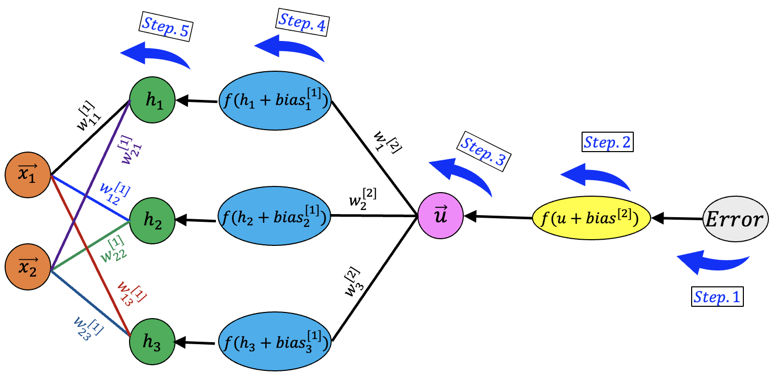
Figure. 22 Backpropagation steps in neural network

\(\textbf {Step.1}\)

In the first step, we should calculate the derivative of the error with respect to the \({\vec{\boldsymbol{y}}}_{predicted}\):

(133)\[{\vec {\boldsymbol{V}}}_{step.1} = \frac {\partial {Error}} {\partial {\boldsymbol{\vec{y}}}_{predicted}} = - \frac {1}{n} [({\boldsymbol{\vec {y}}}_{real}) - ({\boldsymbol{\vec {y}}}_{predicted})]\]

In the above equation, the members of 2 vectros including \({\vec{\boldsymbol{y}}}_{real}\) and \({\vec{\boldsymbol{y}}}_{predicted}\) should be deducted in an element-wise manner. Note that the \({\vec {\boldsymbol{V}}}_{step.1}\) is a \(n\)-dimensional vector.

\(\textbf {Step.2}\)

In this step, we should take derivative of the \({\vec{\boldsymbol{y}}}_{predicted}\) with respect to the \({\vec{u}}^{[b]}\). To this end, we should calculate the derivative of the \(\textbf{Sigmoid Function}\). The derivative of the \(\textbf{Sigmoid Function}\) is calculated as:

(134)\[\frac {\partial f(x)}{\partial x} = f(x) \times [1-f(x)]\]

Now we can write:

(135)\[\frac {\partial {\vec{\boldsymbol{y}}}_{predicted}} {\partial {\vec{\boldsymbol{u}}}^{[b]}}= \begin{gathered} \begin{bmatrix} f({u^{[b]}}_{11}) & f({u^{[b]}}_{12}) & f({u^{[b]}}_{13}) & f({u^{[b]}}_{14}) \end{bmatrix} \end{gathered} \odot \begin{gathered} \begin{bmatrix} (1-f({u^{[b]}}_{11})) & (1-f({u^{[b]}}_{12})) & (1-f({u^{[b]}}_{13})) & (1-f({u^{[b]}}_{14})) \end{bmatrix} \end{gathered}\]

Note

The \(\odot\) defines the element-wise multiplication.

So far, we have reached to the \({\vec{\boldsymbol{u}}}^{[b]}\) where we have:

(136)\[{\vec {\boldsymbol{V}}}_{step.2} = \frac {\partial Error}{\partial {\vec{\boldsymbol{u}}}^{[b]}} = \frac {\partial Error}{\partial {\vec{\boldsymbol{y}}}_{predicted}} \odot \frac {\partial {\vec{\boldsymbol{y}}}_{predicted}}{\partial {\vec{\boldsymbol{u}}}^{[b]}} = {\vec {\boldsymbol{V}}}_{step.1} \odot \frac {\partial {\vec{\boldsymbol{y}}}_{predicted}}{\partial {\vec{\boldsymbol{u}}}^{[b]}}\]

In the above equation, the first term on the right hand-side was obtained in the Equation.133 and the second term was found in Equation.135.

Note that the \({\partial Error}/{\partial {\vec{\boldsymbol{u}}}^{[b]}}\) is a \(n\)-dimensional vector.

\(\textbf {Step.3}\)

At this step, we move one more step backward to get to the \(\boldsymbol{h^{[b \Rightarrow a]}}\). The purpose is to calculate the \({\partial Error} / {\partial \boldsymbol{h^{[b \Rightarrow a]}}}\):

(137)\[{{\boldsymbol{V}}}_{step.3} = \frac{{\partial Error}} {\partial \boldsymbol{h^{[b \Rightarrow a]}}} = \frac {\partial{\vec{\boldsymbol{u}}}^{[b]}}{\partial \boldsymbol{h^{[b \Rightarrow a]}}} \frac{\partial Error}{\partial {\vec{\boldsymbol{u}}}^{[b]}}\]

According to the Equation.128, the first term in the right hand-side of the above equation, is equal to \({\vec{\boldsymbol{W}}}^{[2]}\). In addition, the second term in the right hand-side of the above equation was found in Equation.136

Note that the \({\vec{\boldsymbol{W}}}^{[2]}\) is a \([r \times 1]\) vector and the \({\vec{\boldsymbol{V}}}_{step.2}\) is a \([1 \times n]\) vector. Thus, the \({\vec{\boldsymbol{V}}}_{step.3}\) is a \([r \times n]\) matrix.

There are two more local gradient that we need to calculate in this step:

\(\textbf {1. }\) \({\partial Error} / {\partial \vec{\boldsymbol{W}}^{[2]}}\)

In order to calculate the above derivative, using chain rule we can write:

(138)\[\frac{{\partial Error}} {{\partial \vec{\boldsymbol{W}}^{[2]}}} = \frac{{\partial Error}} {\partial {\vec{\boldsymbol{u}}}^{[b]}} \frac{\partial {\vec{\boldsymbol{u}}}^{[b]}} {\partial \vec{\boldsymbol{W}}^{[2]}}\]

The first term in the right hand-side of the above equation was obtained in Equation.136. In addition, according to the Equation.128, the second term in the right hand-side of the above equation, is equal to \(\boldsymbol{h^{[b \Rightarrow a]}}\). Please note that the \({\partial Error} / {\partial \vec{\boldsymbol{u}^{[b]}}}\) is a \([1 \times n]\) vector. This vector should be multiplied by \(\boldsymbol{h^{[b \Rightarrow a]}}\) and as this is a \([r \times n]\) matrix, for calculation of Equation.138, we should reshape the \(\boldsymbol{h^{[b \Rightarrow a]}}\) by transposing it. To be more specific, for the \(\boldsymbol{h^{[b \Rightarrow a]}}\), we should consider a \([n \times r]\) matrix instead.

Finally, the output of the \({\partial Error} / {\partial \vec{\boldsymbol{W}}^{[2]}}\) is a \([1 \times r]\) vector.

Note

In general, as the \(\vec{\boldsymbol{W}}^{[2]}\) is a \(r\)-dimensional vector, the \({{\partial Error}} / {{\partial \vec{\boldsymbol{W}}^{[2]}}}\) is also a \(r\)-dimensional vector

\(\textbf {2. }\) \({\partial Error} / {\partial {bias^{[2]}}}\)

In order to calculate the above derivative, using chain rule we can write:

(139)\[\frac{{\partial Error}} {{\partial {bias^{[2]}}}} = \frac{{\partial Error}} {\partial {\vec{\boldsymbol{u}}}^{[b]}} \frac{\partial {\vec{\boldsymbol{u}}}^{[b]}} {\partial {bias}^{[2]}}\]

Again, the first term in the right hand-side of the above equation was obtained in Equation.136. Furthermore, according to the Equation.130, the second term in the right hand-side of the above equation is a \(n\)-dimensional vector where all \(n\) elements are equal to 1.

Note

In general, as the \(bias^{[2]}\) is a scalar, the \({{\partial Error}}/ {{\partial {bias}^{[2]}}}\) is also a scalar

According to the above note, we need to calculate the inner product of 2 vectors on the right-hand side of the Equation.139. Now we can re-write the Equation.139:

(140)\[\frac{{\partial Error}} {{\partial {bias^{[2]}}}} = \sum_{i=0}^n [ \frac{{\partial Error}} {\partial {\vec{\boldsymbol{u}}}^{[b]}}]_{i}\]

\(\textbf {Step.4}\)

Here we move another step backward to calculate the \({{\partial Error}} / {{\partial {h^{[b]}}}}\):

(141)\[{{\boldsymbol{V}}}_{step.4} = \frac{{\partial Error}} {{\partial {h^{[b]}}}} = \frac{{\partial Error}} {\partial {\boldsymbol{h}}^{[b \Rightarrow a]}} \odot \frac{{\partial {\boldsymbol{h}}^{[b \Rightarrow a]}}} {\partial {\boldsymbol{h}}^{[b]}}\]

The first term in the right hand-side of the above equation was obtained in Equation.137. In addition, based on Equation.126 we can write the second term on the right-hand side as following:

(142)\[\begin{split}\frac{{\partial {\boldsymbol{h}}^{[b \Rightarrow a]}}} {\partial {\boldsymbol{h}}^{[b]}} = \begin{gathered} \begin{bmatrix} f({h^{[b]}}_{11}) \quad & f({h^{[b]}}_{12}) \quad & f({h^{[b]}}_{13}) \quad & f({h^{[b]}}_{14}) \\ f({h^{[b]}}_{21}) \quad & f({h^{[b]}}_{22}) \quad & f({h^{[b]}}_{23}) \quad & f({h^{[b]}}_{24}) \\ f({h^{[b]}}_{31}) \quad & f({h^{[b]}}_{32}) \quad & f({h^{[b]}}_{33}) \quad & f({h^{[b]}}_{34}) \end{bmatrix} \end{gathered} \odot \begin{gathered} \begin{bmatrix} (1-f({h^{[b]}}_{11})) \quad & (1-f({h^{[b]}}_{12})) \quad & (1-f({h^{[b]}}_{13})) \quad & (1-f({h^{[b]}}_{14})) \\ (1-({h^{[b]}}_{21})) \quad & (1-f({h^{[b]}}_{22})) \quad & (1-f({h^{[b]}}_{23})) \quad & (1-f({h^{[b]}}_{24})) \\ (1-f({h^{[b]}}_{31})) \quad & (1-f({h^{[b]}}_{32})) \quad & (1-f({h^{[b]}}_{33})) \quad & (1-f({h^{[b]}}_{34})) \end{bmatrix} \end{gathered}\end{split}\]

Finally, the \({{\boldsymbol{V}}}_{step.4}\) is a \([r \times n]\) matrix.

\(\textbf {Step.5}\)

In the last step of the Backpropagation we should calculate \({{\partial Error}} / {\partial \boldsymbol{W^{[1]}}}\):

(143)\[ \frac {{\partial Error}}{\partial \boldsymbol{W^{[1]}}} = \frac {{\partial Error}} {\partial {\boldsymbol{h}}^{[b]}} \frac {{\partial {\boldsymbol{h}}}^{[b]}} {\partial \boldsymbol{W^{[1]}}}\]

The first term in the right hand-side of the above equation was obtained in Equation.141 which is the same thing found in the Step.4.

In addition, the second term on the right-hand side of the above equation is found based on Equation.121 which is equal to \(\boldsymbol{X}\). It should be noted that \(\boldsymbol{V_{step.4}}\) is a \([r \times n]\) matrix tht should be multiplied by \(\boldsymbol{X}\) which is a \([d \times n]\) matrix. In order to perform this matrix multiplication, we require to reshape the \(\boldsymbol{X}\) by transposing it. to have a \([n \times d]\) matrix instead.

Finally, the \({{\partial Error}} / {\partial \boldsymbol{W^{[1]}}}\) is a \([r \times d]\) matrix.

Note

In general, as the \(\boldsymbol{W^{[1]}}\) is a matrix, the \({{\partial Error}}/ {\partial \boldsymbol{W^{[1]}}}\) is also a matrix with the same dimensions

Next, we should calculate \({{\partial Error}} / {\partial {\vec{\boldsymbol{bias}}}^{[1]}}\):

(144)\[ \frac {{\partial Error}}{\partial {\vec{\boldsymbol{bias}}}^{[1]}} = \frac {{\partial Error}} {\partial {\boldsymbol{h}}^{[b]}} \odot \frac {{\partial {\boldsymbol{h}}}^{[b]}} {\partial {\vec{\boldsymbol{bias}}}^{[1]}}\]

Again, the first term in the right hand-side of the above equation was obtained in Equation.141 which is the same thing found in the Step.4. In addition, the second term on the right-hand side of the above equation is found based on Equation.121 which is equal to:

(145)\[\begin{split} \frac {{\partial {\boldsymbol{h}}}^{[b]}} {\partial {\vec{\boldsymbol{bias}}}^{[1]}}= \begin{gathered} \begin{bmatrix} 1 \quad & 1 \quad & 1 \quad & 1 \\ 1 \quad & 1 \quad & 1 \quad & 1 \\ 1 \quad & 1 \quad & 1 \quad & 1 \\ \end{bmatrix} \end{gathered}\end{split}\]

According to the above equation, the \({{\partial Error}} / {\partial {\vec{\boldsymbol{bias}}}^{[1]}}\) is obtained by \(\textbf {row-wise inner product }\) of the \({{\partial Error}} / {\partial {\boldsymbol{h}}^{[b]}}\) and \({{\partial {\boldsymbol{h}}}^{[b]}} / {\partial {\vec{\boldsymbol{bias}}}^{[1]}}\) that yields to:

(146)\[\begin{split} \frac {{\partial Error}}{\partial {\vec{\boldsymbol{bias}}}^{[1]}}= \begin{gathered} \begin{bmatrix} \sum\limits_{i=0}^n (\frac {{\partial Error}} {\partial {\boldsymbol{h}}^{[b]}})_{1i}\\ \sum\limits_{i=0}^n (\frac {{\partial Error}} {\partial {\boldsymbol{h}}^{[b]}})_{2i} \\ \sum\limits_{i=0}^n (\frac {{\partial Error}} {\partial {\boldsymbol{h}}^{[b]}})_{3i} \end{bmatrix} \end{gathered}\end{split}\]

7.5. Update weights and biases

As you remember, we initialized the values of the \(\boldsymbol{W^{[1]}}\), \({\vec{\boldsymbol{bias}}}^{[1]}\), \({\vec{\boldsymbol{W}}}^{[2]}\) and \({bias}^{[2]}\) by generating random numbers. Now we should used \(\textbf {Gradient Descent}\) method to update these values to be used in the next round of training our neural network in the Feedforward process.

\(\textbf {Gradient Descent}\)

(147)\[ \begin{align}\begin{aligned} {\boldsymbol{W^{[1]}}}_{current} = {\boldsymbol{W^{[1]}}}_{previous} - \lambda \frac {{\partial Error}}{\partial {\boldsymbol{W^{[1]}}}_{previous}}\\ {\vec{\boldsymbol{bias}}}^{[1]}_{current} = {{\vec{\boldsymbol{bias}}}^{[1]}}_{previous} - \lambda \frac {\partial Error}{\partial {{\vec{\boldsymbol{bias}}}^{[1]}}_{previous}}\\ {\vec{\boldsymbol{W}}}^{[2]}_{current} = {{\vec{\boldsymbol{W}}}^{[2]}}_{previous} - \lambda \frac {\partial Error}{\partial {{\vec{\boldsymbol{W}}}^{[2]}}_{previous}}\\ {{bias}^{[2]}}_{current} = {{bias}^{[2]}}_{previous} - \lambda \frac {\partial Error}{\partial {{bias}^{[2]}}_{previous}}\end{aligned}\end{align} \]

In the above equations, the \(\lambda\) is the \(\textbf {Learning Rate}\). Meanwhile, the deduction of the vectors and matrices should be done in an element-wise fashion.

7.6. C++ code from scratch

Now it is the time to implement the above algorithm in a computer code. The C++ is chosen here due to its speed which is an important parameter when it comes to dealing with a computational problem like training a neural network.

For the sake of simplicity, as described in the previous sections, we consider 4 input data each of which includes 2 dimensions. There is also one value associated to every single input data which are actual values that we want to predict by training our neural network. Our neural network consists of 1 hidden layer with 3 neurons.

Note

There are many different libraries having the neural network implemented and ready to use in a bunch of lines of code. Although, they all are advantageous to use in terms of saving time but implementation of the algorithm from the scratch, gives much better and deeper understanding regarding how a neural network actually works.

The different blocks of the code will be explained as following:

The first step is including standard required headers:

#include <random>
#include <vector>
#include <iostream>
#include <cmath>
#include <fstream>

using namespace std;

Then we should define our input data and assigned target values (That we want to finally predict):

vector<vector<double>> input_data = {{ 0,0 },{ 0,1 },{ 1,0 },{ 1,1 }};
vector<double> target_values = {0,1,1,0};

Next, we should define the architecture of the neural network including the number of data, number of neurons in the hidden layer, number of dimensions that each input data has and the learning rate:

int number_of_data = 4;
int dimensions = 2;
int hidden_layer_nodes = 3;
double lr = 1;

We should set up the engine for producing random numbers between 0 and 1 to fill the weights matrix/vector:

random_device rd;
default_random_engine eng(rd());
uniform_real_distribution<> distr{0, 1};

The number of the training iteration should be defined here:

int training_iteration = 5000;

Now, we should define the required vectors and matrices in the Feedforward process:

vector<vector<double>> weights_1;
vector<double> weights_2;

vector<vector<double>> matrix_x;

vector<double> bias_1 ;
vector<double> bias_2 ;

vector<vector<double>> hidden_values;
vector<vector<double>> hidden_values_activated;
vector<vector<double>> hidden_values_activated_derivative;

vector<double> output_values;
vector<double> output_values_activated;

There are also some vectors and matrices which are required in the Backpropagation that need to be defined:

vector<double> front_output_activated;
vector<double> behind_output_activated;

vector<vector<double>> Gradient_wrt_W_2;
vector<double> Calculate_Grad_W2_Vector;
vector<double> Calculate_Grad_Bias1_Vector;
vector<vector<double>> BP_behind_hidden_activated;

vector<vector<double>> Gradient_wrt_W_1;
vector<vector<double>> BP_front_hidden_activated;
vector<vector<double>> Calculate_Grad_W1_Matrix;

We need to initialize the above vectors and matrices with values using Vectors_Matrices_Builder function. It should be noted that the weights vector/matrix should be filled with random numbers and the rest of the defined items should be filled with 0 elements:

void Vectors_Matrices_Builder(){

   for (int i = 0 ; i < hidden_layer_nodes ; i++){
     weights_2.push_back(distr(eng));
     weights_1.push_back(vector<double>());
       for (int j  = 0 ; j < dimensions ; j++){
           weights_1[i].push_back(distr(eng));
       }
   }
   for (int i = 0 ; i < hidden_layer_nodes ; i++){

     bias_1.push_back(0);
     Calculate_Grad_Bias1_Vector.push_back(0);
   }
   .
   .
   .
   .

We define a class Required_Functions containing some required function including the Sigmoid function, derivative of the Sigmoid function and the Prediction function so we can have access to these function in different sections of out implementation:

 class Required_Functions{
  public:

  double sigmoid (double x ){
        return  1/(1+exp(-x));
  }

  double derivative_sigmoid (double x ){
        return  sigmoid(x)*(1-sigmoid(x));
  }

double predict (vector<double> Input_to_Predict , vector<vector<double>> W1,vector<double> W2, vector<double> bias1 , double bias2){

vector<double> W1X;
vector<double> W1X_activated;

 for (int m = 0 ; m < hidden_layer_nodes ; m++){

 double result_hidden_layer = 0;
 .
 .
 .
 .

We need to define two more vectors to store the values of the errors and iteration of the training:

vector<double> Training_Number;
vector<double> Error_Values;

Here is the main body of the code where we initialize the vectors and matrices and form the X matrix from the input data:

int main(){

Vectors_Matrices_Builder();

   // Forming the training set
   for (int i = 0 ; i < dimensions ; i++){

      matrix_x.push_back(vector<double>());

         for (int j = 0 ; j < number_of_data ; j++){

            matrix_x[i].push_back(input_data[j][i]);  // dimension x number_of_data (2 x 4)
   }
}

Here is the outermost loop where the first training starts:

for (int epoch = 0 ; epoch < training_iteration ;  epoch++){

The Feedforward process starts by implementation of the 5 steps as mentioned before. The final step is to calculate the predicted values:

for (int m = 0 ; m < hidden_layer_nodes ; m++){

   double result_hidden_layer = 0;

      for (int n = 0 ; n < number_of_data ; n++){

      for (int k = 0 ; k < dimensions ; k++){
.
.
.
.

for (int r = 0 ; r < number_of_data ; r++){

double result_output_layer = 0;

   for (int p = 0 ; p < weights_2.size() ; p++){

     result_output_layer += weights_2[p] * hidden_values_activated[p][r];
   }

     result_output_layer += bias_2[0];

     output_values[r] = result_output_layer ;
     output_values_activated[r] = Function->sigmoid(result_output_layer) ;

     }

After predicting the target values, we should calculate the error:

double error = 0;
   for (int k = 0 ; k < number_of_data ; k++){

      error +=  pow((target_values[k] - output_values_activated[k]), 2 );
   }
   error  = error / (2. * number_of_data);

cout << "In Training Number: " << epoch+1 << " ->" << " The Error is: " << error << endl;

Error_Values.push_back(error);
Training_Number.push_back(epoch);

Having the Feedforward process done, we should start the Backpropagation by implementing the 5 steps as mentioned before:

for (int t = 0 ; t < number_of_data ; t++){
    front_output_activated[t] = (-1. / number_of_data) * (target_values[t] - output_values_activated[t]);
}

for (int w = 0 ; w < number_of_data ; w++){
    behind_output_activated[w] = front_output_activated[w] * Function->derivative_sigmoid(output_values_activated[w]);
}
.
.
.
.

We need to update the weights and biases using Gradient Descent approach at the end of the Backpropagation:

////////////////////////// UPDATE W2 ////////////////////////////////////

for (int i = 0 ; i < hidden_layer_nodes ; i++){

weights_2[i] = weights_2[i] - lr * Calculate_Grad_W2_Vector[i];
}
////////////////////////// UPDATE Bias2 ////////////////////////////////////

bias_2[0] = bias_2[0] - lr * new_bias2;

////////////////////////// UPDATE W1 ////////////////////////////////////

for (int i = 0 ; i < hidden_layer_nodes ; i++){

for (int j = 0 ; j < dimensions ; j++){

weights_1[i][j] = weights_1[i][j] - lr * Calculate_Grad_W1_Matrix[i][j];

}
}
////////////////////////// UPDATE Bias1 ////////////////////////////////////

for (int i = 0 ; i < hidden_layer_nodes ; i++){

bias_1[i] = bias_1[i] - lr * Calculate_Grad_Bias1_Vector[i];
}

Here we save the results in a text file including 2 columns corresponding to the number of the iteration in training of the neural network and the calculated error at that iteration respectively:

string filename("Results-CPP.txt");
fstream file_out;
file_out.open(filename, std::ios::out);

for (int r=0 ; r < training_iteration; r++){

    file_out << Training_Number[r] << "       " << Error_Values[r] << endl;
};

file_out.close();

After finishing the training procedure, at the end, we can print out the predicted value for an input data to assess the performance of out neural network:

vector<double> Predict_value = { 1,0 };
double prediction = Function->predict(Predict_value, weights_1 , weights_2 , bias_1 , bias_2[0]);

cout << endl ;
cout << "The predicted Value is: " << prediction << endl;

The output of the above code will be:

In Training Number: 1 -> The Error is: 0.132078
In Training Number: 2 -> The Error is: 0.130562
In Training Number: 3 -> The Error is: 0.129356
In Training Number: 4 -> The Error is: 0.128402
In Training Number: 5 -> The Error is: 0.127652
.
.
.
.
In Training Number: 4997 -> The Error is: 0.000122601
In Training Number: 4998 -> The Error is: 0.000122501
In Training Number: 4999 -> The Error is: 0.000122401
In Training Number: 5000 -> The Error is: 0.000122301

The predicted Value is: 0.984482

According to the above output, it is clear that the error starting at around 0.13 in the first iteration, gradually decreases to nearly 0 at the last training iteration. The neural network does a good job in predicting the input value where we get a number fairly close to 1 which is what we expect for this input number.

If we change the input value to predict as following:

vector<double> Predict_value = { 1,1 };
double prediction = Function->predict(Predict_value, weights_1 , weights_2 , bias_1 , bias_2[0]);

cout << endl ;
cout << "The predicted Value is: " << prediction << endl;

The output of the code will be like this:

,
,
,
,
In Training Number: 4997 -> The Error is: 8.65583e-05
In Training Number: 4998 -> The Error is: 8.64981e-05
In Training Number: 4999 -> The Error is: 8.64379e-05
In Training Number: 5000 -> The Error is: 8.63779e-05

The predicted Value is: 0.00975805

Again, we get a value small enough and close to 0 which is what we expected for this input value.

We can, investigate the performance of the neural network based on the number of the neurons in the hidden layer:

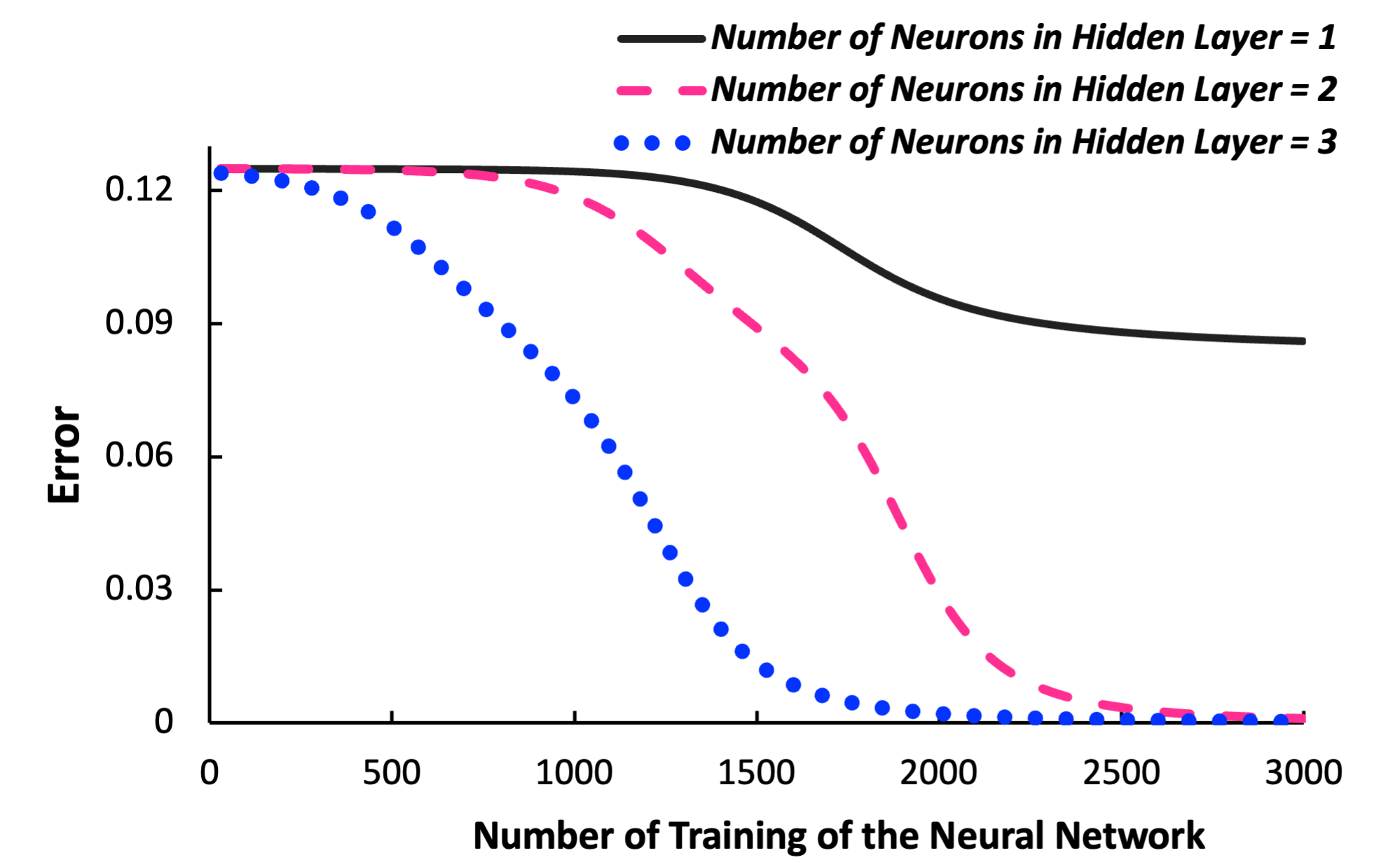
Figure. 23 Performance of the neural network based on the number of neurons

We can clearly see that increasing the neurons inside the hidden layer boosts the accuracy of the model by reducing the error. However, it should be noted that it will come at the cost of increasing the computational cost.

The complete C++ code is presented as following:

#include <random>
#include <vector>
#include <iostream>
#include <cmath>
#include <fstream>

using namespace std;


vector<vector<double>> input_data = {{ 0,0 },{ 0,1 },{ 1,0 },{ 1,1 }};
vector<double> target_values = {0,1,1,0};

int number_of_data = 4;
int dimensions = 2;
int hidden_layer_nodes = 3;
// Defining learning rate
double lr = 1;

random_device rd;
default_random_engine eng(rd());
uniform_real_distribution<> distr{0, 1};


int training_iteration = 5000;

///////////////// Required Vectors/Matrices for Feed Forward /////////////////

vector<vector<double>> weights_1;
vector<double> weights_2;

vector<vector<double>> matrix_x;

vector<double> bias_1 ;
vector<double> bias_2 ;

vector<vector<double>> hidden_values;
vector<vector<double>> hidden_values_activated;
vector<vector<double>> hidden_values_activated_derivative;

vector<double> output_values;
vector<double> output_values_activated;

///////////////// Required Vectors/Matrices for Back Propagation /////////////////

vector<double> front_output_activated;
vector<double> behind_output_activated;

vector<vector<double>> Gradient_wrt_W_2;
vector<double> Calculate_Grad_W2_Vector;
vector<double> Calculate_Grad_Bias1_Vector;
vector<vector<double>> BP_behind_hidden_activated;

vector<vector<double>> Gradient_wrt_W_1;
vector<vector<double>> BP_front_hidden_activated;
vector<vector<double>> Calculate_Grad_W1_Matrix;

////////////////////////////////////////////////////////////////////

void Vectors_Matrices_Builder(){

   for (int i = 0 ; i < hidden_layer_nodes ; i++){
      weights_2.push_back(distr(eng));
      weights_1.push_back(vector<double>());
      for (int j  = 0 ; j < dimensions ; j++){
            weights_1[i].push_back(distr(eng));
      }
   }

   for (int i = 0 ; i < hidden_layer_nodes ; i++){

      bias_1.push_back(0);
      Calculate_Grad_Bias1_Vector.push_back(0);
   }

   bias_2.push_back(0);

   for (int i = 0 ; i < number_of_data ; i++){

      output_values.push_back(0);
      output_values_activated.push_back(0);

      front_output_activated.push_back(0);
      behind_output_activated.push_back(0);
   }

   for (int i = 0 ; i < hidden_layer_nodes ; i++){

      hidden_values.push_back(vector<double>());
      hidden_values_activated.push_back(vector<double>());
      hidden_values_activated_derivative.push_back(vector<double>());

      BP_front_hidden_activated.push_back(vector<double>());
      BP_behind_hidden_activated.push_back(vector<double>());

      for (int j = 0 ; j < number_of_data ; j++){
            hidden_values[i].push_back(0);
            hidden_values_activated[i].push_back(0);
            BP_front_hidden_activated[i].push_back(0);
            hidden_values_activated_derivative[i].push_back(0);
            BP_behind_hidden_activated[i].push_back(0);
      }
   }

   for (int i = 0 ; i < number_of_data ; i++){

      Gradient_wrt_W_2.push_back(vector<double>());

      for (int j = 0 ; j < hidden_layer_nodes ; j++){
            Gradient_wrt_W_2[i].push_back(0);
      }
   }

   for (int j = 0 ; j < hidden_layer_nodes ; j++){
            Calculate_Grad_W2_Vector.push_back(0);
      }


   for (int i = 0 ; i < number_of_data ; i++){

      Gradient_wrt_W_1.push_back(vector<double>());

      for (int j = 0 ; j < dimensions ; j++){
            Gradient_wrt_W_1[i].push_back(0);
      }
   }

   for (int i = 0 ; i < hidden_layer_nodes ; i++){

      Calculate_Grad_W1_Matrix.push_back(vector<double>());

      for (int j = 0 ; j < dimensions ; j++){
            Calculate_Grad_W1_Matrix[i].push_back(0);
      }
   }
}
/////////////////////// Defines required function including sigmoid, derivative of the sigmoid and prediction ///////////////////////////////////////////////

class Required_Functions{
   public:

   double sigmoid (double x ){
         return  1/(1+exp(-x));
   }

   double derivative_sigmoid (double x ){
         return  sigmoid(x)*(1-sigmoid(x));
   }

double predict (vector<double> Input_to_Predict , vector<vector<double>> W1,vector<double> W2, vector<double> bias1 , double bias2){

vector<double> W1X;
vector<double> W1X_activated;

   for (int m = 0 ; m < hidden_layer_nodes ; m++){

   double result_hidden_layer = 0;

      for (int n = 0 ; n < 1 ; n++){

      for (int k = 0 ; k < dimensions ; k++){

      result_hidden_layer += W1[m][k] * Input_to_Predict[k];  // 3x1 Output
      }
      //derivatives_matrix_y_predict[m] = derivative_sigmoid(result);

      result_hidden_layer += bias1[m];

      W1X.push_back(result_hidden_layer) ;
      W1X_activated.push_back(sigmoid(result_hidden_layer)) ;
      }
   }

   double result_output = 0;
   for (int m = 0 ; m < hidden_layer_nodes ; m++){
      result_output += W2[m] * W1X_activated[m];
      }
      result_output += bias2;

   return sigmoid(result_output);
}
};

Required_Functions Start;
Required_Functions *Function = &Start;

///////////////////////////////////////////////////
vector<double> Training_Number;
vector<double> Error_Values;
////////////////////////////////////////////////////

int main(){

Vectors_Matrices_Builder();

   // Forming the training set
   for (int i = 0 ; i < dimensions ; i++){

      matrix_x.push_back(vector<double>());

         for (int j = 0 ; j < number_of_data ; j++){

            matrix_x[i].push_back(input_data[j][i]);  // dimension x number_of_data (2 x 4)
   }
}

/////////////////////////// Training Begins! ////////////////////////////////////

for (int epoch = 0 ; epoch < training_iteration ;  epoch++){

/////////////////////////// Feed Forwards //////////////////////////

/////////////////////////// W_1 * X //////////////////////////////

   for (int m = 0 ; m < hidden_layer_nodes ; m++){

   double result_hidden_layer = 0;

      for (int n = 0 ; n < number_of_data ; n++){

      for (int k = 0 ; k < dimensions ; k++){

      result_hidden_layer += weights_1[m][k] * matrix_x[k][n];
      }

      result_hidden_layer += bias_1[m];

      hidden_values[m][n]= result_hidden_layer ;
      hidden_values_activated[m][n]= Function->sigmoid(result_hidden_layer) ;
      result_hidden_layer = 0;

      }
   }

/////////////////////////// W_2 * SIGMOID (W_1 * X) ////////////////////////////////////

for (int r = 0 ; r < number_of_data ; r++){

   double result_output_layer = 0;

      for (int p = 0 ; p < weights_2.size() ; p++){

      result_output_layer += weights_2[p] * hidden_values_activated[p][r];
      }

      result_output_layer += bias_2[0];

      output_values[r] = result_output_layer ;
      output_values_activated[r] = Function->sigmoid(result_output_layer) ;

      }

/////////////////////////// Error Calculation //////////////////////////

double error = 0;
   for (int k = 0 ; k < number_of_data ; k++){

      error +=  pow((target_values[k] - output_values_activated[k]), 2 );
   }
   error  = error / (2. * number_of_data);

cout << "In Training Number: " << epoch+1 << " ->" << " The Error is: " << error << endl;

Error_Values.push_back(error);
Training_Number.push_back(epoch+1);

/////////////////////////// Back Propagation //////////////////////////

   for (int t = 0 ; t < number_of_data ; t++){
      front_output_activated[t] = (-1. / number_of_data) * (target_values[t] - output_values_activated[t]);
   }

   for (int w = 0 ; w < number_of_data ; w++){
      behind_output_activated[w] = front_output_activated[w] * Function->derivative_sigmoid(output_values_activated[w]);
   }

/////////////////////////// Form Grad W2 ////////////////////////////////////

for (int r = 0 ; r < number_of_data ; r++){

      for (int p = 0 ; p < hidden_layer_nodes ; p++){

      Gradient_wrt_W_2[r][p] = hidden_values_activated[p][r];
      }
}
/////////////////////////// Calculation Grad(W2)) ////////////////////////////////////

for (int r = 0 ; r < hidden_layer_nodes ; r++){

   double result_1 = 0;

      for (int p = 0 ; p < number_of_data ; p++){

      result_1 += behind_output_activated[p] * Gradient_wrt_W_2[p][r];
      }

      Calculate_Grad_W2_Vector[r] = result_1 ;
      }
/////////////////////////// Calculation Grad(bias2)) ////////////////////////////////////

double new_bias2 = 0;

for (int r = 0 ; r < number_of_data ; r++){
      new_bias2 += behind_output_activated[r];
   }

/////////////////////////// Moving in front of hidden_activated ///////////////////////////

/////////////////////////// W2 * behind_output_activated ////////////////////////////////////

for (int r = 0 ; r < hidden_layer_nodes ; r++){

      for (int p = 0 ; p < number_of_data ; p++){

      BP_front_hidden_activated[r][p] = weights_2[r] * behind_output_activated[p];
      }
}

/////////////////////////// Derivative of hidden values activated ////////////////////////////////////

for (int r = 0 ; r < hidden_layer_nodes ; r++){

      for (int p = 0 ; p < number_of_data ; p++){

      hidden_values_activated_derivative[r][p] =  Function->derivative_sigmoid(hidden_values[r][p]);
      }
}
/////////////////////////// Moving behind hidden_activated ///////////////////////////

///////////////// (W2 * behind_output_activated) * (Derivative of hidden values activated) ////////////////////

for (int r = 0 ; r < hidden_layer_nodes ; r++){

      for (int p = 0 ; p < number_of_data ; p++){

      BP_behind_hidden_activated[r][p] =  BP_front_hidden_activated[r][p] * hidden_values_activated_derivative[r][p];
      }

}

////////////////////////// Form Grad W1 ////////////////////////////////////

for (int r = 0 ; r < dimensions ; r++){

      for (int p = 0 ; p < number_of_data ; p++){

      Gradient_wrt_W_1[p][r] = matrix_x[r][p];
      }
}

/////////////////////////// Calculation Grad(W1)) ////////////////////////////////////

   for (int m = 0 ; m < hidden_layer_nodes ; m++){

   double result_4 = 0;

      for (int n = 0 ; n < dimensions ; n++){

      for (int k = 0 ; k < number_of_data ; k++){

      result_4 += BP_behind_hidden_activated[m][k] * Gradient_wrt_W_1[k][n];
      }

      Calculate_Grad_W1_Matrix[m][n]= result_4 ;
      result_4 = 0;

      }
   }
/////////////////////////// Calculation Grad(bias1)) ////////////////////////////////////

   for (int i = 0 ; i < hidden_layer_nodes ; i++){

      double new_bias1 = 0;

      for (int j = 0 ; j < number_of_data ; j++){

         new_bias1 += BP_behind_hidden_activated[i][j];
      }

      Calculate_Grad_Bias1_Vector[i] = new_bias1;
   }

////////////////////////// Gradient Descent ////////////////////////////////////
////////////////////////// UPDATE W2 ////////////////////////////////////

for (int i = 0 ; i < hidden_layer_nodes ; i++){

weights_2[i] = weights_2[i] - lr * Calculate_Grad_W2_Vector[i];
}
////////////////////////// UPDATE Bias2 ////////////////////////////////////

bias_2[0] = bias_2[0] - lr * new_bias2;

////////////////////////// UPDATE W1 ////////////////////////////////////

for (int i = 0 ; i < hidden_layer_nodes ; i++){

for (int j = 0 ; j < dimensions ; j++){

weights_1[i][j] = weights_1[i][j] - lr * Calculate_Grad_W1_Matrix[i][j];

}
}
////////////////////////// UPDATE Bias1 ////////////////////////////////////

for (int i = 0 ; i < hidden_layer_nodes ; i++){

bias_1[i] = bias_1[i] - lr * Calculate_Grad_Bias1_Vector[i];
}
}

////////////////////////// Saving in a text file ////////////////////////////////////

   string filename("Results-CPP.txt");
   fstream file_out;
   file_out.open(filename, std::ios::out);

   for (int r=0 ; r < training_iteration; r++){

      file_out << Training_Number[r] << "       " << Error_Values[r] << endl;
   };

   file_out.close();
////////////////////////// Prediction ////////////////////////////////////

vector<double> Predict_value = { 1,1 };
double prediction = Function->predict(Predict_value, weights_1 , weights_2 , bias_1 , bias_2[0]);

cout << endl ;
cout << "The predicted Value is: " << prediction << endl;

      return 0 ;
   }

7.7. Classification of an eye disease

Now we can test our neural network for prediction of an eye disease where the posterior of the eye globe becomes flattened. This eye disorder is called IIH and more details are available in Chapter 6 (Please check out Section 6.3). We have information of 661 eye globes in which 301 of them have been identified as flattened eye globes. In other words, those are the eyes having IIH syndrome. The rest of the data, are healthy eyes where the curvature of the eye globe is normal. We have saved the data in a text file (EYE-DATA.txt) as following :

0.05,0.25,0.04,0.2,0.1,1,0.3333333333,1,0.33325,1
0.05,0.1,0.04,0.2,0.1,0.3333333333,0.3333333333,0.6665,0.1,1
0.05,0.25,0.04,0.2,1,1,1,1,0.6665,1
.
.
.
1,0.25,1,1,1,1,0.3333333333,0.1,0.33325,0
1,0.25,1,1,1,0.3333333333,1,0.1,0.33325,0
1,0.25,1,0.04,1,0.3333333333,0.3333333333,0.1,0.1,0

Note

The EYE-DATA.txt file is available inside the Neural-Network repository.

In the above data, each line corresponds to the information of a single eye. There are 10 numbers in each line separated with ,. The first 7 numbers are the normalized stiffness of the 7 tissues within the optic nerve head, the \(8^{th}\) and \(9^{th}\) are the normalized Intraocular Pressure (IOP) and Intracranial Pressure (ICP) respectively. With that being said, every single input data has 9 dimensions. Finally, the \(10^{th}\) is a number which is either 0 or 1. The 0 means that the eye does not have IIH while if it is 1, it indicates that this is a flattened eye globe.

We use, these data to train our neural network. Finally, the purpose is giving a new input to our neural network and predict if this eye globe with these specific properties is flattened or not.

The main body of the code for training the neural network code is almost the same as presented before in Section 7.6. However there are some modifications. First of all, we need to update the number_of_data and dimensions:

int number_of_data = 661;
int dimensions = 9;

In addition, we require to read the data from the text file that could be done as following:

vector<vector<double>> input_data ;
vector<double> target_values ;
.
.
.
int main(){

//////////////////////////////////////////////////////
vector <vector <string> > data;
 ifstream infile( "EYE-DATA.txt" );
 string line;
 string str;

 //  Read the file
 while (getline(infile, line))
 {   istringstream ss (line);
     vector <string> record;

     while (getline(ss, str, ','))
         record.push_back(str);
     data.push_back (record);
 }

 for (int i = 0 ; i < number_of_data ; i++){

   input_data.push_back(vector<double>());
   target_values.push_back(stod(data[i][9]));

     for (int j  = 0 ; j < dimensions ; j++){

         input_data[i].push_back(stod(data[i][j]));

     }
 }

This prediction is performed at the end of training using this block of code:

vector<double> Predict_value1 = {0.05,0.25,0.2,0.2,0.1,1,0.3333333333,1,0.33325};
vector<double> Predict_value2 = {1,0.11,1,0.03,1,0.22,0.3333333333,0.1,0.11};

double prediction1 = Function->predict(Predict_value1, weights_1 , weights_2 , bias_1 , bias_2[0]);
double prediction2 = Function->predict(Predict_value2, weights_1 , weights_2 , bias_1 , bias_2[0]);

cout << endl ;
cout << "The prediction for the first eye is: " << prediction1 << endl;
cout << "The prediction for the second eye is: " << prediction2 << endl;

Please note that, the first two lines, are the information of two new eyes that did NOT exist in the original data set.

.
.
.
In Training Number: 4997 -> The Error is: 6.3865e-06
In Training Number: 4998 -> The Error is: 6.38371e-06
In Training Number: 4999 -> The Error is: 6.38093e-06
In Training Number: 5000 -> The Error is: 6.37814e-06

The prediction for the first eye is: 0.997147
The prediction for the second eye is: 0.00195323

The above results indicate that the first eye was identified as a flattened globe and the second eye, was classified as an healthy eye. These predictions are correct as after performing a FEM analysis, it turned out that the first eye based the given properties is deformed in a way that the globe becomes flattened while the second eye keeps its normal shape indicating an healthy eye.

Note

The full C++ code is available inside the Neural-Network repository (IIH_Prediction_Neural_Network.cpp)