2. Multi-Physics Problem

Note

The reader is encouraged to look at this paper to make a sense out of numerical solution of a coupled physics problem:

2.1 Coupled System of Equations

In this section, we solve a coupled system of partial differential equations. To be more specific, we look into the Poisson-Nernst-Planck equations representing coupled physics including the chemical and electrical fields.

The strong from of the Nernst-Planck equations is expressed as:

(79)\[\frac{\partial c}{\partial t}+ \nabla . (-D_i \nabla c_i- z_i \mu_i F c_i \nabla \phi)=0,\quad i=Na^+,Cl^-\]

Where \(c\) is concentration of the mobile species, \(D\) is diffusion constant of the mobile species, \(\mu = \frac{D}{RT}\) is mobility of the ionic species ,:math:R is universal gas constant , \(T\) is temperature, \(F\) is Faraday constant and \(\phi\) is Electrical potential.

(80)\[\nabla^2 \phi = -\frac{F}{\varepsilon_0 \varepsilon_r}(z_{Na} c_{Na} + z_{Cl} c_{Cl} + z_{fixed} c_{fixed})\]

The approximate solution is sought on scalar spaces including \(S^{(c)}\) and \(S^{(\phi)}\) corresponding to the function spaces representing the concentration of the ions and electric potential respectively.

(81)\[ \begin{align}\begin{aligned} S^{c}=span \{\omega_0^{c} ,...,\omega_N^{c} \}\\ S^{\phi}=span \{\lambda_0^{\phi} ,...,\lambda_N^{\phi} \}\end{aligned}\end{align} \]

The \(\omega_i\) and \(\lambda_i\) are the basis functions which are linearly independent. This approximation is used to discretize the problem in space. In this regard the approximate solution and can be expressed as a linear combination of the basis functions:

(82)\[ \begin{align}\begin{aligned} c= \sum_{j=0}^N \alpha_j \omega_j (x,y)\\ \phi= \sum_{j=0}^N \beta_j \lambda_j (x,y)\end{aligned}\end{align} \]

The coefficients \(\alpha_i\) and \(\beta_i\) should be computed. A mixed scalar space is then defined as: \(\textbf{S} = S^{(c)} \times S^{(\phi)}\) along with a test function \(\textbf{v} = (v_c,v_{\phi})\) .The test functions are chosen as \(\forall v_c , v_{\phi} \in \textbf{S}\), So we can define the test function: \(v_c = \omega_i\) and \(v_{\phi} = \lambda_i\) . In order to derive the weak form of the NP equation, we should multiply it by \(v_c\):

(83)\[ \int_{\Omega} v_c [\frac{\partial c}{\partial t}+ \nabla . (-D \nabla c- z \mu F c \nabla \phi)]dx\]

Then the above equation could be expanded as following:

(84)\[ \int_{\Omega} v_c \frac{\partial{c}}{\partial t} dx+\int_{\Omega} v_c D {\nabla}^2{c} dx - \int_{\Omega} v_c \mu F z \nabla{c} \nabla{\phi} dx -\int_{\Omega} v_c \mu F z {\nabla}^2{\phi} dx = 0\]

By integration by part and applying the divergence theorem, it yields to:

(85)\[ \begin{align}\begin{aligned} \int_{\Omega} v_c \frac{\partial c}{\partial t} dx - \int_{\partial \Omega} v_c D \nabla{c}.n.ds +\\ \int_{\Omega} D(\nabla c.\nabla \phi) dx-\int_{\Omega} v_c \mu Fz \nabla{c} \nabla{\phi} dx -\\ \int_{\partial \Omega} v_c \mu Fzc \nabla{\phi}.n.ds+\int_{\Omega} \mu Fz \nabla(cv_c).\nabla \phi.dx=0\end{aligned}\end{align} \]

In the above equation, \(n\) is the outward normal vector on the boundaries. The terms including \(ds\) correspond to the Neumann boundary condition that vanish as they are equal to zero:

(86)\[ \begin{align}\begin{aligned} \int_{\Omega} v_c \frac{\partial c}{\partial t} dx + \int_{\Omega} D(\nabla c.\nabla \phi) dx-\\ \int_{\Omega} v_c \mu Fz \nabla{c} \nabla{\phi} dx +\int_{\Omega} v_c \mu F(\nabla c.\nabla\phi)dx+ \int_{\Omega} \mu Fcz \nabla(v_c).\nabla\phi.dx=0\end{aligned}\end{align} \]

In the above equation, the third and fourth terms cancel out:

(87)\[ \int_{\Omega} v_c \frac{\partial c}{\partial t}dx+\int_{\Omega}D(\nabla c.\nabla v_c)dx+\int_{\Omega} \mu zcF(\nabla{\phi}.\nabla{v_c})dx = 0\]

The derivative in time could be written according to the backward-Euler scheme:

(88)\[ \frac{\partial c}{\partial t} = \frac{c-c^0}{\Delta t}\]

Then after plugging into the equation.87:

(89)\[ \int_{\Omega} v_c c dx-\int_{\Omega}v_c c^0 dx+\Delta t \int_{\Omega}D(\nabla c.\nabla{v_c})dx+\Delta t \int_{\Omega}\mu z Fc (\nabla \phi.\nabla{v_c})dx=0\]

The same approach could be taken by deriving the weak form of the Poisson equation after multiplying it into a test function \(v_{\phi}\):

(90)\[ \int_{\Omega} v_{\phi}\nabla^2 \phi dx = -\int_{\Omega} v_{\phi} [-\frac{F}{\varepsilon_0 \varepsilon_r}(z_{Na} c_{Na} + z_{Cl} c_{Cl} + z_{fixed} c_{fixed})]dx\]

After integration by part and applying the divergence theorem, it yields to:

(91)\[\int_{\partial \Omega} v_{\phi}\nabla \phi n.ds -\int_{\Omega} \nabla v_{\phi}.\nabla \phi dx = \int_{\Omega} v_{\phi} [-\frac{F}{\varepsilon_0 \varepsilon_r}(z_{Na} c_{Na} + z_{Cl} c_{Cl} + z_{fixed} c_{fixed})]dx\]

The first term in the left-hand side of the above equation, corresponds to the Neumann boundary condition that is equal to zero. So, this could be rewritten by expanding the right-hand side to find the final weak from of the Poisson equation:

(92)\[ \begin{align}\begin{aligned} \int_{\Omega} \nabla v_{\phi} \nabla \phi dx - \int_{\Omega} v_{\phi} \frac{F}{\varepsilon_0 \varepsilon_r}(z_{Na} c_{Na})dx-\\ \int_{\Omega} v_{\phi} \frac{F}{\varepsilon_0 \varepsilon_r}(z_{Cl} c_{Cl})dx - \int_{\Omega} v_{\phi} \frac{F}{\varepsilon_0 \varepsilon_r}(z_{fixed} c_{fixed})dx = 0\end{aligned}\end{align} \]

The constants used in the simulation as well as the initial conditions are presented in below tables:

Table 1 Constants

\(F(\frac{c}{mol})\)	\(\epsilon_0(\frac{F}{m})\)	\(\epsilon_r\)	\(z_{Na}\)	\(z_{Cl}\)	\(z_{fixed}\)	\(R(\frac{J}{mol.K})`\)	\(T(K)\)	\(D_{Na}(\frac{m^2}{s})\)	\(D_{Cl}(\frac{m^2}{s})\)
96487	\(8.85 \times 10^{-12}\)	100	1	-1	-1	8.3114	293	\(10^{-7}\)	\(10^{-7}\)

Table 2 Initial Condition

Solution	Gel
\(c_{Na}=1mM\)	\(c_{Na}=5.193mM\)
\(c_{Cl}=1mM\)	\(c_{Cl}=0.193mM\)
	\(c_{fixed}=1mM\)

2.2 Finite Element Implementation

Note

In this section we replicate the results in this paper

The summary of the FEM code implemented in FeniCS is presented here:

from dolfin import *

Then we should define the constants:

# Diffusion constant for Na+ cations GEL
D_Na = 1.0 * (10 ** (-7.))

# Diffusion constant for Cl- anioins GEL
D_Cl = 1.0 * (10 ** (-7.))

# Diffusion constant for Na+ cations SOLUTION
D_Na_s = 1.0 * (10 ** (-7.))

# Diffusion constant for Cl- anioins SOLUTION
D_Cl_s = 1.0 * (10 ** (-7.))

# The gas constant
R = 8.31

# Initial value for Na+ in the solution
c_init_Na_sol = 1

# Initial value for Cl- in the solution
c_init_Cl_sol = 1

# Initial value for fixed anioin (e.g. bound charge) in the gel
c_init_Fixed_gel = 5


c_init_Na_gel = ((c_init_Fixed_gel + pow(c_init_Fixed_gel ** 2 + 4 * pow(c_init_Cl_sol, 2), 0.5))) / 2.
c_init_Cl_gel = ((-c_init_Fixed_gel + pow(c_init_Fixed_gel ** 2 + 4 * pow(c_init_Cl_sol, 2), 0.5))) / 2.


# Valence of Na+
z_Na = 1.0

# Valence of Cl-
z_Cl = -1.0

# Valence of Fixed anioin
z_Fixed = -1.0

# Anion concentration
# C_0 = Constant(500.0)
eps_vacume = 8.85 * pow(10, -12)
eps_water = 100.
eps_sclera = 100.

# Dielectric permittivity
epsilon = eps_vacume * eps_water
epsilon_p = eps_vacume * eps_sclera

# Temperature
Temp = 293.0

# Electrical mobility for Na+ cations
mu_Na = D_Na / (R * Temp)

# Electrical mobility for Cl- cations
mu_Cl = D_Cl / (R * Temp)

mu_Na_s = D_Na_s / (R * Temp)

# Electrical mobility for Cl- cations
mu_Cl_s = D_Cl_s / (R * Temp)

# Faraday number
Faraday = 96485.34

Next we should present the mesh in the simulation. The domains include a hydrogel (Shown in red color with the dimensions of \(4 \times 10 mm^2\)) placed in the middle of a solution domain (Shown in green color with the dimensions of \(50 \times 50 mm^2\)). The mesh was created in the GMSH.

Note

The density of the element should be significantly increased near the boundaries of the hydrogel and solution to capture the steep gradient of the concentration of the mobile ions

The domains and the mesh are shown here:

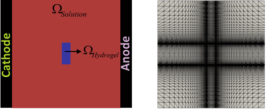
Figure. 11 Computational Domains (Left) and Mesh (Right)

Note

The mesh file is available in the github repository in the folder PNP-MESH.

mesh = Mesh()
hdf = HDF5File(mesh.mpi_comm(), "0file.h5", "r")
hdf.read(mesh, "/mesh", False)
subdomains = MeshFunction('size_t', mesh, mesh.topology().dim())

hdf.read(subdomains, "/subdomains")
boundaries = MeshFunction('size_t', mesh, mesh.topology().dim() - 1)
hdf.read(boundaries, "/boundaries")

The integration symbol \(dx\) is defined as:

dx = Measure('dx', domain=mesh, subdomain_data=subdomains)

Next we should define the appropriate element and then form the mixed-function space containing all unknowns:

# Defining element for scalar variables (e.g. concentrations and voltage)
Element1 = FiniteElement("CG", mesh.ufl_cell(), 1)

# Defining the mixed function space
W_elem = MixedElement([Element1, Element1, Element1])

W = FunctionSpace(mesh, W_elem)

The summary of the FEniCS code is presented here:

from dolfin import *

# Diffusion constant for Na+ cations GEL
D_Na = 1.0 * (10 ** (-7.))

# Diffusion constant for Cl- anioins GEL
D_Cl = 1.0 * (10 ** (-7.))

# Diffusion constant for Na+ cations SOLUTION
D_Na_s = 1.0 * (10 ** (-7.))

# Diffusion constant for Cl- anioins SOLUTION
D_Cl_s = 1.0 * (10 ** (-7.))

# The gas constant
R = 8.31

# Initial value for Na+ in the solution
c_init_Na_sol = 1

# Initial value for Cl- in the solution
c_init_Cl_sol = 1

# Initial value for fixed anioin (e.g. bound charge) in the gel
c_init_Fixed_gel = 5

############################
############################
c_init_Na_gel = ((c_init_Fixed_gel + pow(c_init_Fixed_gel ** 2 + 4 * pow(c_init_Cl_sol, 2), 0.5))) / 2.
c_init_Cl_gel = ((-c_init_Fixed_gel + pow(c_init_Fixed_gel ** 2 + 4 * pow(c_init_Cl_sol, 2), 0.5))) / 2.

##############################
##############################
# Valence of Na+
z_Na = 1.0

# Valence of Cl-
z_Cl = -1.0

# Valence of Fixed anioin
z_Fixed = -1.0

# Anion concentration
# C_0 = Constant(500.0)
eps_vacume = 8.85 * pow(10, -12)
eps_water = 100.
eps_sclera = 100.

# Dielectric permittivity
epsilon = eps_vacume * eps_water
epsilon_p = eps_vacume * eps_sclera

# Temperature
Temp = 293.0

# Electrical mobility for Na+ cations
mu_Na = D_Na / (R * Temp)

# Electrical mobility for Cl- cations
mu_Cl = D_Cl / (R * Temp)

mu_Na_s = D_Na_s / (R * Temp)

# Electrical mobility for Cl- cations
mu_Cl_s = D_Cl_s / (R * Temp)

# Faraday number
Faraday = 96485.34

mesh = Mesh()
hdf = HDF5File(mesh.mpi_comm(), "0file.h5", "r")
hdf.read(mesh, "/mesh", False)
subdomains = MeshFunction('size_t', mesh, mesh.topology().dim())

hdf.read(subdomains, "/subdomains")
boundaries = MeshFunction('size_t', mesh, mesh.topology().dim() - 1)
hdf.read(boundaries, "/boundaries")

# File("domains.pvd") << subdomains
# lable domain
dx = Measure('dx', domain=mesh, subdomain_data=subdomains)
.
.
.

# Varitional form for the Nernst-Planck equation in the hydrogel domain for Na+ and Cl-
Weak_NP_Na = ...
Weak_NP_Cl = ...

# Varitional form for the Poisson equation in the hydrogel domain for Na+ and Cl- and fixed charge
Weak_Poisson = ...

##################################

# Varitional form for the Nernst-Planck equation in the solution domain for Na+ and Cl-
Weak_NP_Na_sol = ...

Weak_NP_Cl_sol = ...

# Varitional form for the Poisson equation in the solution domain for Na+ and Cl- and fixed charge
Weak_Poisson_sol = ...

# Summing up variational forms
F = Weak_NP_Na + Weak_NP_Cl + Weak_Poisson + Weak_NP_Cl_sol + Weak_NP_Na_sol + Weak_Poisson_sol

.
.
.

Na_Ion = File("Na.pvd")
Cl_Ion = File("Cl.pvd")
Voltage = File("phi.pvd")

while t <= T:
    bc_left_volt = DirichletBC(W.sub(2), -0.1, boundaries, 35)
    bc_right_volt = DirichletBC(W.sub(2), 0.1, boundaries, 36)
    bcs = [bc_left_volt, bc_right_volt, bc_left_c, bc_right_c, bc_left_c_1, bc_right_c_1]

    J = derivative(F, z, dz)

    problem = NonlinearVariationalProblem(F, z, bcs, J)
    solver = NonlinearVariationalSolver(problem)
    solver.solve()

    (c_Na, c_Cl, phi) = z.split(True)

    C_previous_Na.assign(c_Na)
    C_previous_Cl.assign(c_Cl)

    t += dt


    Na_Ion << c_Na
    Cl_Ion << c_Cl
    Voltage << phi

The results could be visualized in Paraview. Here are the results after 10s for the concentration of the sodium ion, chloride ion and electrical voltage:

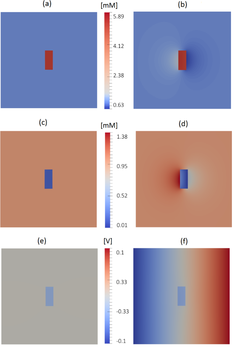
Figure. 12 Initial and stationary solutions

The figures (a), (c) and (e) correspond to the initial values of the \(c_{Na}\) , \(c_{Cl}\) and \(\phi\) respectively. The figures (b), (d) and (f) correspond to the stationary values of the \(c_{Na}\) , \(c_{Cl}\) and \(\phi\) respectively.

Note

The above code has been written with the capability for parallel computation. You can significantly increase the speed if running it in parallel.

In order to run the code in parallel, all you need to do is just opening the terminal and then run this command:

mpirun -np 4 python3 code.py

Where 4 is the number of the cores you want to use to run the code. You can increase it based on number of the cores you have access to.

Note

The complete FEniCS code is available upon request (Please refer to the section : About the Author)