1. Hyperelasticity

Note

The reader is encouraged to look at these resources to get started:

1. Material Models in Continuum Solid Mechanics

2. Finite element implementation of incompressible, transversely isotropic hyperelasticity

3. FEBio: Finite Elements for Biomechanics

4. Applied Mechanics of Solids

1.1 Introduction

The strain energy function \(W\) is defined as:

(1)\[ W=W(I_1 (\textbf {C})),I_2 (\textbf {C})),I_3 (\textbf {C}))\]

In the above equations, \(\textbf {C}\) is the right Cauchy deformation tensor:

(2)\[\textbf {C}=F^TF\]

Where \(F\) is the deformation gradient tensor: \(F=I+\nabla u\). The Jacobian of \(F\) is defined as its determinant: \(J= \lvert F \rvert\).

The \(I_1 (\textbf {C})\), \(I_2 (\textbf {C})\) and \(I_3 (\textbf {C})\) are the invariants of the \(\textbf {C}\) tensor.

(3)\[ \begin{align}\begin{aligned}I_1=tr(\textbf{C})\\I_2=0.5[(tr \textbf{C})^2-tr(\textbf{C}^2)]\\I_3=det (\textbf{C})\end{aligned}\end{align} \]

The second Piola-Kirchhoff stress is defined as:

(4)\[S=2 \frac{\partial W}{\partial \textbf {C}}\]

After applying the chain rule, we can write the term \(\frac{\partial W}{\partial \textbf {C}}\) as:

(5)\[\frac{\partial W}{\partial \textbf {C}}=\frac{\partial W}{I_1} \frac{\partial I_1}{\textbf {C}} + \frac{\partial W}{I_2} \frac{\partial I_2}{\textbf {C}}+\frac{\partial W}{I_3} \frac{\partial I_3}{\textbf {C}}\]

The first term on the right hand side, we could apply the chain rule to calculate the \(\frac{\partial I_1}{\partial C}\):

(6)\[\frac{\partial I_1}{\partial C}=\frac{\partial (I_1)_{11}}{C_{ij}} e_i \otimes e_j + \frac{\partial (I_1)_{22}}{C_{ij}} e_i \otimes e_j + \frac{\partial (I_1)_{33}}{C_{ij}} e_i \otimes e_j\]

Note

The \(e_i\) and \(e_j\) are unit vectors, \(\otimes\) represents the outer product and \(e_i \otimes e_j =0\) if \(i \neq j\).

(7)\[\frac{\partial I_1}{\partial C}=e_1 \otimes e_1 +e_2 \otimes e_2 +e_3 \otimes e_3 = \textbf{I}\]

Similarly we can can derive the \(\frac{\partial I_2}{\partial C}\) and \(\frac{\partial I_3}{\partial C}\):

(8)\[ \begin{align}\begin{aligned}\frac{\partial I_2}{\partial \textbf {C}}= I_1 \textbf {I} - \textbf {C}\\\frac{\partial I_3}{\partial \textbf {C}}= I_2 \textbf {I} - I_1 \textbf {C} + \textbf {C}^2\end{aligned}\end{align} \]

By plugging back the Equation.7 and Equation.8 into the Equation.5, we can find the second piola kirchhoff stress as:

(9)\[\textbf {S}= 2 \alpha_1 \textbf {I} + 2 \alpha_2 \textbf {C} + 2 \alpha_3 \textbf {C}^2\]

In Equation.9:

(10)\[ \begin{align}\begin{aligned}\alpha_1 = \frac{\partial W}{\partial I_1} + \frac{\partial W}{\partial I_2} I_1 + \frac{\partial W}{\partial I_3} I_2\\\alpha_2 = -\frac{\partial W}{\partial I_2} - \frac{\partial W}{\partial I_3} I_1\\\alpha_3 = \frac{\partial W}{\partial I_3}\end{aligned}\end{align} \]

The Cauchy stress is defined as:

(11)\[\sigma = J^{-1} F F^T \textbf {S}\]

Similar to the Equation.1 we can define:

(12)\[ W=W(I_1 (\textbf {b})),I_2 (\textbf {b})),I_3 (\textbf {b}))\]

Where \(\textbf {b}\) is the left Cauchy deformation tensor:

(13)\[\textbf {b}=FF^T\]

It should be noted that the invariants of the \(\textbf {b}\) are obtained similar to the Equation.3. By taking the same steps shown in the Equation.6 and Equation.7

In addition, we take advantage of Cayley-Hamilton theorem:

(14)\[\textbf{b}^3-I_1 \textbf{b}^2+I_2 \textbf{b} - I_3 \textbf{I} =0\]

So the term \(\frac{\partial I_3}{\partial \textbf {b}}\) could be rewritten again:

(15)\[\frac{\partial I_3}{\partial \textbf {b}}= I_3 \textbf {b}^{-1}\]

We can write the \(\frac{\partial W}{\partial \textbf {b}}\):

(16)\[\frac{\partial W}{\partial \textbf {b}}= (\frac{\partial W}{\partial I_1} + \frac{\partial W}{\partial I_2} I_1) \textbf {I} - \frac{\partial W}{\partial I_2}\textbf {b} +\frac{\partial W}{\partial I_3} I_3 \textbf {b}^{-1}\]

After multiplying the \(\textbf {b}\) tensor into the Equation.16 and then by substitution in Equation.11, the stress could be defined as following:

(17)\[ \sigma=\beta_1 \textbf {I}+\beta_2 \textbf {b}+\beta_3 \textbf {b}^2\]

In the above equation:

(18)\[ \begin{align}\begin{aligned}\beta_1 = 2J^{-1} (\frac{\partial W}{\partial I_3}I_3)\\\beta_2 = 2J^{-1} (\frac{\partial W}{\partial I_1} + \frac{\partial W}{\partial I_2} I_1)\\\beta_3 = 2J^{-1} (-\frac{\partial W}{\partial I_2})\end{aligned}\end{align} \]

1.2 Fully Incompressible Model

1.2.1 Constitutive Equations

For the incompressible Neo-Hookean material, the strain energy function is defined as:

(19)\[W=c_1(I_1-3)\]

For the uniaxial tension, the deformation gradient tensor is expressed as:

(20)\[\begin{split} F=\begin{bmatrix} \lambda_1 & 0 & 0\\0 & \lambda_2 & 0\\0 & 0 & \lambda_3\end{bmatrix}\end{split}\]

Considering the equation.19 and with respect to equation.17 and equation.18 then we can calculate the \(\beta_1\), \(\beta_2\) and \(\beta_3\):

(21)\[ \begin{align}\begin{aligned} \beta_1 = 0\\ \beta_2 = 2J^{-1}c_1\\ \beta_3 = 0\end{aligned}\end{align} \]

In the above equation \(c_1= \frac {\mu}{2}\) where \(\mu\) is the shear modulus. In addition for a fully compressible material, \(J= 1\) so \(\beta_2=\mu\) . According to the equation.20 and equation.13 we can calculate the \(\textbf{b}\) as following:

(22)\[\begin{split} \textbf{b}=\begin{bmatrix} {\lambda_1}^2 & 0 & 0\\0 & {\lambda_2}^2 & 0\\0 & 0 & {\lambda_3}^2 \end{bmatrix}\end{split}\]

Then we can write the stress as:

(23)\[\begin{split} \begin{bmatrix} \sigma_{11} & 0 & 0\\0 & 0& 0\\0 & 0 & 0\end{bmatrix} = \beta_{2}\begin{bmatrix} \lambda_{1}^2 & 0 & 0\\0 & \lambda_{2}^2& 0\\0 & 0 & \lambda_{3}^2\end{bmatrix}\end{split}\]

It results in 2 equations:

(24)\[ \begin{align}\begin{aligned}\sigma_{11}=\beta_2 \lambda_{1}^2\\0=\beta_2 \lambda_{2}^2\end{aligned}\end{align} \]

By subtracting the above equations:

(25)\[ \sigma_{11}=(\lambda_{1}^2-\lambda_{2}^2)\beta_{2}\]

It should be noted that in the uniaxial stretch, the stretches in different directions are:

(26)\[\begin{split} \lambda_1=\lambda\\ \lambda_2=\lambda_3= \frac{1}{\sqrt{\lambda}}\end{split}\]

Then the final form of the stress is presented in this form:

(27)\[ \sigma_{11}=\mu(\lambda^2-\frac{1}{\lambda})\]

For the Biaxial tension, the deformation gradients tensor is defined as:

(28)\[\begin{split} F=\begin{bmatrix} \lambda & 0 & 0\\0 & \lambda & 0\\0 & 0 & \frac {1}{\lambda^2}\end{bmatrix}\end{split}\]

As \(\beta_1\) and \(\beta_3\) are equal to zero, after calculating the \(\textbf{b}\) tensor we can write the Equation.17 in this form:

(29)\[\begin{split} \begin{bmatrix} \sigma_{11} & 0 & 0\\0 & \sigma_{22} & 0\\0 & 0 & 0\end{bmatrix}= \beta_1 \begin{bmatrix} \lambda^2 & 0 & 0\\0 & \lambda^2 & 0\\0 & 0 & \frac{1}{\lambda^4}\end{bmatrix}\end{split}\]

It results in 2 equations:

(30)\[\begin{split} \sigma_{11}= \beta_2 \lambda^2\\ 0= \beta_2 \frac{1}{\lambda^4}\end{split}\]

By subtracting the above equations:

(31)\[ \sigma_{11}= \mu (\lambda^2-\frac{1}{\lambda^4})\]

Note

Alternative Way

The stress is defined as following:

(32)\[ \sigma= \alpha_1 \lambda_i^{2} + \alpha_{-1} \lambda_i^{-2}-p\]

Where:

(33)\[\begin{split} \alpha_1= 2 \frac{\partial W}{\partial I_1}\\ \alpha_{-1}= -2 \frac{\partial W}{\partial I_2}\end{split}\]

The parameter \(p\) is defined as hydrostatic pressure:

(34)\[ p= \alpha_1 \frac{1}{\lambda_1^{2} \lambda_2^{2}}+\alpha_{-1}\lambda_1^{2} \lambda_2^{2}\]

We can find \(\alpha_1\) and \(\alpha_{-1}\) : \(\alpha_1=2c_1=\mu\) and \(\alpha_{-1}=0\)

By combining the Equation.32 and Equation.34:

(35)\[ \sigma_{ii}= \mu \lambda_{i}^2-\mu (\frac {1}{\lambda_i^{2}\lambda_i^{2}})\]

Which is same as Equation.31.

1.2.2 Finite Element Implementation

For the fully incompressible Neo-Hookean material the Jacobian of the deformation gradient tensor is unity (e.g. \(J=1\)). The strain energy function is defined as follows:

(36)\[ W= c_1(I_1-3)+p(J-1)\]

Note

In the above equation, the parameter \(p\) is Lagrange Multiplier enforcing the fully incompressibility condition

The stress is defined:

(37)\[ \sigma=\alpha_1 b + \alpha_{-1} b^{-1} - p I\]

Then the stress term is reduced to:

(38)\[ \sigma=\mu b - p I\]

Note

When we solve for a fully incompressible material, we should define our problem on a mixed space including a scalar space (to solve for the \(p\)) and a vector space (to solve for the displacement)

The analytical solution for the uniaxial stretch for different shear modulus could be obtained using this code:

lamda = [0.15,0.2,0.25,0.3,0.35,0.4,0.45,0.5,0.55,0.6,0.65,0.7,0.75,0.8,0.85,0.9,0.95,1.,1.25,1.5,1.75,2,2.25,2.5,2.75,3,3.25,3.5,3.75,4,4.25,4.5,4.47,5]

# Shear modulus = 0.5 MPa
sigma_05 = []
# Shear modulus = 1.5 MPa
sigma_15 = []
# Shear modulus = 3.5 MPa
sigma_35 = []

for i in range (len(lamda)):

        a = 0.5 * (pow(lamda[i], 2) - 1. /(lamda[i]))
        b = 1.5 * (pow(lamda[i], 2) - 1. /(lamda[i]))
        c = 3.5 * (pow(lamda[i], 2) - 1. /(lamda[i]))

        sigma_05.append(a)
        sigma_15.append(b)
        sigma_35.append(c)

import matplotlib.pyplot as plt
print (sigma_05)
plt.xlabel(r'$\mathrm{Stretch}$', fontsize=20)
plt.ylabel(r'$\mathrm{\sigma_{xx}(MPa)}$', fontsize=20)

plt.plot(lamda,sigma_05,  linestyle='-', linewidth=4, color='maroon',label=r'$(\mu=0.5)$')
plt.plot(lamda,sigma_15,  linestyle='-', linewidth=4, color='r',label=r'$(\mu=1.5)$')
plt.plot(lamda,sigma_35,  linestyle='-', linewidth=4, color='teal',label=r'$(\mu=3.5)$')
lg=plt.legend(ncol=1, loc=2, fontsize=15)
axes = plt.gca()
axes.set_xlim([0,5])
axes.set_ylim([-15, 30])

axes.set_yticks([-15,-10,-5,0,5,10,15,20,25,30,35])
axes.set_xticks([0,1,2,3,4,5])

plt.tick_params(axis='both', which='major', labelsize=15)
plt.grid()
plt.show()

The implementation in FEniCS is presented in this code:

from dolfin import *

# Defining Stretches
stretch = [0.15,0.2,0.25,0.3,0.35,0.4,0.45,0.5,0.55,0.6,0.65,0.7,0.75,0.8,0.85,0.9,0.95,1.,1.25,1.5,1.75,2,2.25,2.5,2.75,3,3.25,3.5,3.75,4,4.25,4.5,4.47,5]
BC = []

for x in range(len(stretch)):
              N = stretch[x] - 1.0
              BC.append(N)

tol = 1E-14
# Define boundaries
def FRONT(x, on_boundary):
              return on_boundary and abs(x[2] - 1.0) < tol


# Defining the mesh which is a single hexahedron element
mesh = UnitCubeMesh.create(1,1,1,CellType.Type.hexahedron)

############################################
#element for pressure field
Element1 = FiniteElement("CG", mesh.ufl_cell(), 1)
#element for displacement field
Element2 = VectorElement("CG", mesh.ufl_cell(), 2)

# Defining the mixed function space
W_elem = MixedElement([Element1, Element2])
W = FunctionSpace(mesh, W_elem)
#############################################

boundaries = MeshFunction('size_t', mesh, mesh.topology().dim()-1)
subdomains = MeshFunction('size_t', mesh, mesh.topology().dim())


# Defining integration symbols
dx = Measure('dx', domain=mesh, subdomain_data=subdomains, metadata={'quadrature_degree': 15})
ds = Measure('ds', domain=mesh, subdomain_data=boundaries, metadata={'quadrature_degree': 15})


## Define variational problem
dw = TrialFunction(W)            # Incremental displacement
v  = TestFunction(W)
w = Function(W)
p,u = split(w)

#Definig some continuum mechanics relations
d = u.geometric_dimension()
I = Identity(d)             # Identity tensor
F = I + grad(u)             # Deformation gradient
C = F.T*F                   # Right cauchy stress tensor
b = F*F.T                   # Left cauchy stress tensor
Ib = tr(b)                  # First invariant of b tensor
J  = det(F)                 # Jacobian of deformation gradient tensor

# Shear modulus
mu = 0.5e6

# Strain energy function for fully incompressible model
psi = mu/2.*(Ib - 3.)*dx - p*(J - 1)*dx

# Gateaux derivative in the direction of the test function
F1 = derivative(psi, w, TestFunction(W))

# Compute Jacobian of F
Jac = derivative(F1, w, TrialFunction(W))

sigma_11 = []

def border(x, on_boundary):
              return on_boundary

bound_x =  Expression(("t*x[0]"), degree=1, t=0)

for i in range(len(BC)):

              bound_x.t = BC[i]

              bc_x = DirichletBC(W.sub(1).sub(0), bound_x, border)
              bc_front = DirichletBC(W.sub(1).sub(2), Constant((0)), FRONT)

              bc_all = [bc_x,bc_front]

              problem = NonlinearVariationalProblem(F1, w, bc_all, Jac)

              solver = NonlinearVariationalSolver(problem)

              solver.solve()

              (p, u) = w.split(True)

#Stress calculation
              sig = mu * b - p * I
# Defining a tenso function space
              V = TensorFunctionSpace(mesh, 'Lagrange', 1)
# Projection of the stress on the tensor function space
              sig1 = project(sig, V)

              sigma_11.append((sig1.vector().get_local()[0])*0.000001)

print (sigma_11)

#Obtained results for mu = 0.5 MPa#
sigma_05 = [-3.3220833333333144, -2.4800000000022377, -1.968750000000018, -1.6216666666666604, -1.3673214285714232, -1.1699999999999993, -1.0098611111111104, -0.8749999999999992, -0.7578409090909061, -0.6533333334279298, -0.5579807692745585, -0.4692857143072567, -0.3854166666778288, -0.3050000000060496, -0.2269852941210564, -0.15055555555754435, -0.07506578947488027, -7.390848180406038e-13, 0.38124999999999554, 0.7916666666666644, 1.2455357142857126, 1.7499999999999942, 2.309027777777776, 2.924999999888631, 3.5994318181378744, 4.333333333314409, 5.12740384614507, 5.982142857138549, 6.897916666664428, 7.874999999998786, 8.913602941175803, 10.013888888888484, 9.878593176733789, 12.399999999906841]

#Obtained results for mu = 1.5 MPa#
sigma_15 = [-9.966249999999953, -7.4400000000052655, -5.906250000000058, -4.864999999999997, -4.101964285714497, -3.50999999999999, -3.029583333333331, -2.624999999999993, -2.2735227272727245, -1.9599999999999933, -1.6739423078102886, -1.4078571429217734, -1.1562500000334857, -0.9150000000181479, -0.6809558823631715, -0.45166666667263133, -0.2251973684246401, -2.217263493368278e-12, 1.1437499999999825, 2.3749999999999947, 3.7366071428571317, 5.250000000116358, 6.927083333333332, 8.774999999844844, 10.798295454413642, 12.999999999943254, 15.382211538435248, 17.94642857141561, 20.69374999999328, 23.624999999996415, 26.740808823527377, 30.04166666666549, 29.63577953020131, 37.19999999983032]

#Obtained results for mu = 3.5 MPa#
sigma_35 = [-23.254583333333265, -17.360000000015262, -13.781250000000021, -11.351666666666649, -9.571249999999983, -8.189999999999996, -7.069027777155056, -6.124999999999978, -5.304886363636268, -4.573333333994748, -3.9058653849219174, -3.285000000150805, -2.697916666744805, -2.1350000000423432, -1.5888970588473983, -1.0538888889028104, -0.5254605263241604, -5.173676343700641e-12, 2.6687499999999695, 5.5416666666666545, 8.718749999880098, 12.249999999999975, 16.163194443414437, 20.47499999922037, 25.19602272696517, 30.333333333200915, 35.89182692301562, 41.874999999969944, 48.28541666665088, 55.1249999999915, 62.39522058823055, 70.09722222221926, 69.15015223713617, 86.79999999993669]

#Plotting the Results#
import matplotlib.pyplot as plt
plt.xlabel(r'$\mathrm{Stretch}$', fontsize=20)
plt.ylabel(r'$\mathrm{\sigma_{xx}(MPa)}$', fontsize=20)

plt.plot(stretch,sigma_05,  linestyle='-', linewidth=4, color='y',label=r'$(\mu=0.5\/\/MPa)$')
plt.plot(stretch,sigma_15,  linestyle='-', linewidth=4, color='c',label=r'$(\mu=1.5\/\/MPa)$')
plt.plot(stretch,sigma_35,  linestyle='-', linewidth=4, color='k',label=r'$(\mu=3.5\/\/MPa)$')
lg=plt.legend(ncol=1, loc=2, fontsize=15)
axes = plt.gca()
axes.set_xlim([0,5])
axes.set_ylim([-15, 30])

axes.set_yticks([-15,-10,-5,0,5,10,15,20,25,30,35])
axes.set_xticks([0,1,2,3,4,5])

plt.tick_params(axis='both', which='major', labelsize=15)
plt.grid()
plt.show()

The results of analytical solution and finite element implementation are compared in figure.1:

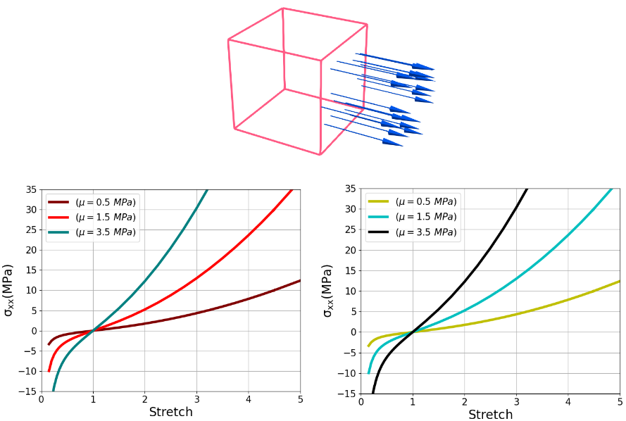
Figure. 1 The stress results for the fully incompressible material model in uniaxial loading - Finite Element (Right) vs Analytical (Left)

The analytical solution for the Biaxial stretch for different shear modulus could be obtained using the code:

lamda = [0.15,0.2,0.25,0.3,0.35,0.4,0.45,0.5,0.55,0.6,0.65,0.7,0.75,0.8,0.85,0.9,0.95,1.,1.25,1.5,1.75,2,2.25,2.5,2.75,3,3.25,3.5,3.75,4,4.25,4.5,4.47,5]

# Shear modulus = 0.5 MPa
sigma_05 = []
# Shear modulus = 1.5 MPa
sigma_15 = []
# Shear modulus = 3.5 MPa
sigma_35 = []

for i in range (len(lamda)):

        a = 0.5 * (pow(lamda[i],2) - 1. /(pow(lamda[i],4)))
        b = 1.5 * (pow(lamda[i], 2) - 1. / (pow(lamda[i], 4)))
        c = 3.5 * (pow(lamda[i], 2) - 1. / (pow(lamda[i], 4)))

        sigma_05.append(a)
        sigma_15.append(b)
        sigma_35.append(c)


import matplotlib.pyplot as plt
print (sigma_05)
plt.xlabel(r'$\mathrm{Stretch}$', fontsize=20)
plt.ylabel(r'$\mathrm{\sigma_{xx}=\sigma_{yy}\/\/(MPa)}$', fontsize=20)

plt.plot(lamda,sigma_05,  linestyle='-', linewidth=4, color='lime',label=r'$(\mu=0.5)$')
plt.plot(lamda,sigma_15,  linestyle='-', linewidth=4, color='m',label=r'$(\mu=1.5)$')
plt.plot(lamda,sigma_35,  linestyle='-', linewidth=4, color='orange',label=r'$(\mu=3.5)$')
lg=plt.legend(ncol=1, loc=2, fontsize=15)
axes = plt.gca()
axes.set_xlim([0,5])
axes.set_ylim([-15, 35])

axes.set_yticks([-15,-10,-5,0,5,10,15,20,25,30,35])
axes.set_xticks([0,1,2,3,4,5])

plt.tick_params(axis='both', which='major', labelsize=15)
plt.grid()
plt.show()

And similarly the implementation of the FEM code in FEniCS is presented here:

from dolfin import *

# Defining Stretches
stretch = [0.15,0.2,0.25,0.3,0.35,0.4,0.45,0.5,0.55,0.6,0.65,0.7,0.75,0.8,0.85,0.9,0.95,1.,1.25,1.5,1.75,2,2.25,2.5,2.75,3,3.25,3.5,3.75,4,4.25,4.5,4.47,5]
BC = []

for x in range(len(stretch)):
         N = stretch[x] - 1.0
         BC.append(N)

tol = 1E-14
# Define boundaries
def LEFT(x, on_boundary):
         return on_boundary and x[0] < tol

def RIGHT(x, on_boundary):
         return on_boundary and abs(x[0] - 1.0) < tol

def BOTTOM(x, on_boundary):
         return on_boundary and x[1] < tol

def TOP(x, on_boundary):
         return on_boundary and abs(x[1] - 1.0) < tol

def FRONT(x, on_boundary):
         return on_boundary and abs(x[2] - 1.0) < tol

def BACK(x, on_boundary):
         return on_boundary and (x[2]) < tol

# Defining the mesh which is a single hexahedron element
mesh = UnitCubeMesh.create(1,1,1,CellType.Type.hexahedron)


#element for pressure field
Element1 = FiniteElement("CG", mesh.ufl_cell(), 1)
#element for displacement field
Element2 = VectorElement("CG", mesh.ufl_cell(), 2)

# Defining the mixed function space
W_elem = MixedElement([Element1, Element2])
W = FunctionSpace(mesh, W_elem)
#############################################

boundaries = MeshFunction('size_t', mesh, mesh.topology().dim()-1)
subdomains = MeshFunction('size_t', mesh, mesh.topology().dim())


# Defining integration symbols
dx = Measure('dx', domain=mesh, subdomain_data=subdomains, metadata={'quadrature_degree': 10})
ds = Measure('ds', domain=mesh, subdomain_data=boundaries, metadata={'quadrature_degree': 10})


## Define variational problem
dw = TrialFunction(W)            # Incremental displacement
v  = TestFunction(W)
w = Function(W)
p,u = split(w)

#Definig some continuum mechanics relations
d = u.geometric_dimension()
I = Identity(d)             # Identity tensor
F = I + grad(u)             # Deformation gradient
C = F.T*F                   # Right cauchy stress tensor
b = F*F.T                   # Left cauchy stress tensor
Ib = tr(b)                  # First invariant of b tensor
J  = det(F)                 # Jacobian of deformation gradient tensor

# Shear modulus
mu = 3.5e6

# Strain energy function for fully incompressible model
psi = mu/2.*(Ib - 3.)*dx - p*(J - 1)*dx

# Gateaux derivative in the direction of the test function
F1 = derivative(psi, w, TestFunction(W))

# Compute Jacobian of F
Jac = derivative(F1, w, TrialFunction(W))

sigma_11 = []
sigma_22 = []


def border(x, on_boundary):
         return on_boundary

bound_x =  Expression(("t*x[0]"), degree=1, t=0)
bound_y =  Expression(("t*x[1]"), degree=1, t=0)

for i in range(len(BC)):

         bound_x.t = BC[i]
         bound_y.t = BC[i]

         bc_x = DirichletBC(W.sub(1).sub(0), bound_x, border)
         bc_y = DirichletBC(W.sub(1).sub(1), bound_y, border)
         bc_front = DirichletBC(W.sub(1).sub(2), Constant((0)), FRONT)

         bc_all = [bc_x,bc_y,bc_front]

         problem = NonlinearVariationalProblem(F1, w, bc_all, Jac)

         solver = NonlinearVariationalSolver(problem)

         solver.solve()

         (p, u) = w.split(True)

#Stress calculation
         sig = mu * b - p * I
# Defining a tensor function space
         Vv = TensorFunctionSpace(mesh, 'Lagrange', 1)
# Projection of the stress on the tensor function space
         sig1 = project(sig, Vv)

         sigma_11.append((sig1.vector().get_local()[0])*0.000001)

print (sigma_11)

#Obtained results for mu = 0.5 MPa#
sigma_05 = [-987.6430709876522, -312.4800000000002, -127.96874999999937, -61.68339506172817, -33.258200229071136, -19.451249999999895, -12.092013222069799, -7.8750000000000036, -5.31285764292055, -3.678024691358014, -2.589772373166203, -1.8374656393169522, -1.2989969135802488, -0.9007031249999968, -0.5965929377042906, -0.35707895137936096, -0.16261883157741178, 8.145274061386054e-17, 0.5764499999999999, 1.0262345679012317, 1.477938879633484, 1.9687500000000013, 2.5117407788446906, 3.1121999999999943, 3.772507427771319, 4.4938271604938125, 5.276768364202937, 6.121668054977084, 7.028721604938255, 7.99804687499999, 9.029717451299652, 10.12378067367779, 9.989197609075557, 12.499199999999991]

#Obtained results for mu = 0.5 MPa#
sigma_15 = [-2962.92921296296, -937.4399999999958, -383.90625000000057, -185.0501851851853, -99.77460068721344, -58.3537499999997, -36.27603966620935, -23.624999999999954, -15.938572928761642, -11.034074074074056, -7.769317119498598, -5.512396917950832, -3.8969907407407285, -2.702109374999993, -1.7897788131128693, -1.0712368541380837, -0.4878564947322365, 3.805590898063224e-16, 1.7293499999999953, 3.0787037037036926, 4.433816638900447, 5.906249999999991, 7.53522233653405, 9.336599999999983, 11.317522283314, 13.48148148148149, 15.830305092608764, 18.365004164931293, 21.08616481481487, 23.994140624999996, 27.089152353899063, 30.371342021033435, 29.967592827226596, 37.49759999999998]

#Obtained results for mu = 0.5 MPa#
sigma_35 = [-6913.501496913527, -2187.3599999999847, -895.7812499999939, -431.78376543209447, -232.8074016034988, -136.15874999999932, -84.6440925544885, -55.12499999999978, -37.19000350044388, -25.746172839506176, -18.128406612163456, -12.862259475218625, -9.092978395061715, -6.304921874999984, -4.176150563930013, -2.499552659655526, -1.1383318210418847, 6.882290512141593e-16, 4.035149999999988, 7.183641975308622, 10.345572157434399, 13.781249999999941, 17.582185451912803, 21.78539999999999, 26.407551994399167, 31.456790123456745, 36.93737854942055, 42.85167638483961, 49.20105123456792, 55.986328124999986, 63.2080221590976, 70.8664647157445, 69.92438326352887, 87.49440000000017]

#Plotting#
import matplotlib.pyplot as plt
#print (sigma_05)
plt.xlabel(r'$\mathrm{Stretch}$', fontsize=20)
plt.ylabel(r'$\mathrm{\sigma_{xx}=\sigma_{yy}\/\/(MPa)}$', fontsize=20)

plt.plot(stretch,sigma_05,  linestyle='-', linewidth=4, color='b',label=r'$(\mu=0.5)$')
plt.plot(stretch,sigma_15,  linestyle='-', linewidth=4, color='g',label=r'$(\mu=1.5)$')
plt.plot(stretch,sigma_35,  linestyle='-', linewidth=4, color='crimson',label=r'$(\mu=3.5)$')
lg=plt.legend(ncol=1, loc=2, fontsize=15)
axes = plt.gca()
axes.set_xlim([0,5])
axes.set_ylim([-15, 35])

axes.set_yticks([-15,-10,-5,0,5,10,15,20,25,30,35])
axes.set_xticks([0,1,2,3,4,5])

plt.tick_params(axis='both', which='major', labelsize=15)
plt.grid()
plt.show()

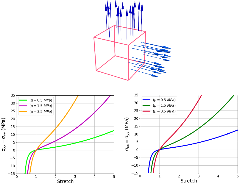
Figure. 2 The stress results for the fully incompressible material model in biaxial loading - Finite Element (Right) vs Analytical (Left)

1.3. Nearly Incompressible Model

1.3.1. Constitutive Equations

For the nearly incompressible Neo-Hookean material, the bulk modulus appears in the strain energy function. It should be noted that as the ratio \(\frac{K}{\mu}\) increases, the behavior of the material becomes closer to a fully incompressible material model (e.g. \(J\) converges to unity).

The strain energy function is defined as:

(39)\[ W=c_1(I_1-3)+ \frac{1}{2}K(Ln(J))^2\]

Where \(I_1\) corresponds to the first invariant of the \(\tilde{C}\) where \(C=J^{\frac{-2}{3}}C\). The stress is defined as:

(40)\[ \sigma=pI+ \frac{2}{J}[c_1 b - \frac{1}{3} (c_1 I_1)I]\]

In the above equation:

(41)\[ p = K \frac{Ln(J)}{J}\]

1.3.2 Finite Element Implementation

The FEniCS implementation of the Neo-Hookean nearly incompressible material on a single hexahedron element under biaxial stretch is shown as below:

from dolfin import *

parameters["form_compiler"]["representation"] = "tsfc"

stretch = [0.95,1.,1.25,1.5,1.75,2,2.25,2.5,2.75,3]

BC = []

for x in range(len(stretch)):
         N = stretch[x] - 1.0
         BC.append(N)

tol = 1E-14

# Define boundary

def FRONT(x, on_boundary):
         return on_boundary and abs(x[2] - 1.0) < tol


mesh = UnitCubeMesh.create(1,1,1,CellType.Type.hexahedron)

############################################
V = VectorFunctionSpace(mesh, 'CG', degree=1)

du  = TrialFunction(V)           # Trial function
v  = TestFunction(V)             # Test function
u  = Function(V)
#############################################

boundaries = MeshFunction('size_t', mesh, mesh.topology().dim()-1)
subdomains = MeshFunction('size_t', mesh, mesh.topology().dim())


dx = Measure('dx', domain=mesh, subdomain_data=subdomains, metadata={'quadrature_degree': 2})
ds = Measure('ds', domain=mesh, subdomain_data=boundaries, metadata={'quadrature_degree': 2})


#################
d = u.geometric_dimension()
I = Identity(d)             # Identity tensor
F = I + grad(u)             # Deformation gradient
C = F.T*F                   # Right cauchy stress tensor
b = F*F.T                   # Left cauchy stress tensor
Ic = tr(C)
J  = det(F)                 # Jacobian of deformation gradient tensor
Ib = tr(b)                  # First invariant of b tensor

Ic_bar = pow(J,-2./3.)*Ic
C_bar = pow(J,-2./3.)*C
B_bar = pow(J,-2./3.)*b

# The bulk modulus (K) and shear modulus (mu) are defined here. Feel free to change them to see the effect of K/mu in the results
mu = 1.5E6
K = 7.5E10

psi = (mu/2. * (Ic_bar - 3.) + 0.5 * K * pow(ln(J),2)) * dx

F1 = derivative(psi, u, v)

# Compute Jacobian of F
Jac = derivative(F1, u, du)

sigma_11 = [] # Array for storing the stress in x direction
sigma_22 = [] # Array for storing the stress in y direction
JJJ = [] # Array for storing the Jacobian

def border(x, on_boundary):
         return on_boundary

bound_x =  Expression(("t*x[0]"), degree=1, t=0)
bound_y =  Expression(("t*x[1]"), degree=1, t=0)


for i in range(len(BC)):


         bound_x.t = BC[i]
         bound_y.t = BC[i]

         bc_x = DirichletBC(V.sub(0), bound_x, border)
         bc_y = DirichletBC(V.sub(1), bound_y, border)
         bc_front = DirichletBC(V.sub(2), Constant((0)), FRONT)


         bc_all = [bc_x,bc_y,bc_front]

         problem = NonlinearVariationalProblem(F1, u, bc_all, Jac)

         solver = NonlinearVariationalSolver(problem)

         solver.solve()

         #sig = inv(J)*(lmbda*ln(J)*I + mu * (b - I))

         sig = (K * ln(J) / J) * I + 2./J * (mu/2. * B_bar - 1./3. * (mu / 2.) * Ic_bar * I)

         S = TensorFunctionSpace(mesh, 'P', 1)

         W = FunctionSpace(mesh, 'P', 1)

         sig1 = project(sig, S)

         JJ = project(J, W)

         JJJ.append((JJ.vector().get_local()[0]))

         sigma_11.append((sig1.vector().get_local()[0])*0.000001)
         sigma_22.append((sig1.vector().get_local()[4])*0.000001)

         File("displacement.pvd") << u

print (sigma_11)
print (sigma_22)
print (JJJ)

Next figure shows how stress – stretch behavior of the model alters as the ratio \(\frac{K}{\mu}\) increases.

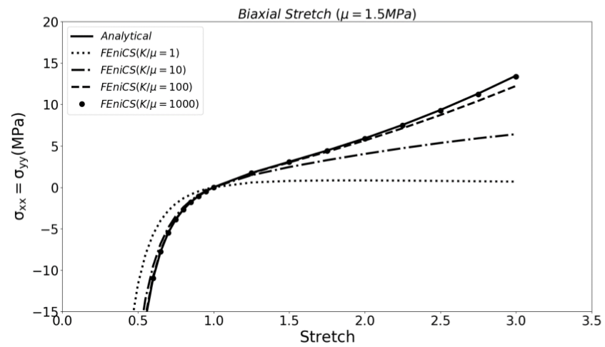
Figure. 3 Effect of compressibility in biaxial tension test– FEM (FEniCS) vs Analytical Solution

The above figure illustrates that when \(\frac{K}{\mu}>100\) the behavior of the model starts converging to the fully incompressible Neo-Hookean model. When \(\frac{K}{\mu}>1000\) the solution is matched with the fully incompressible material model as shown in next figure:

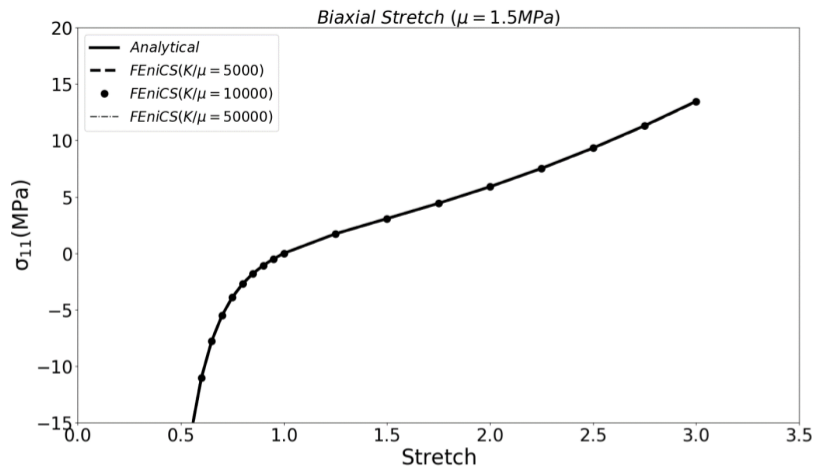
Figure. 4 Nearly incompressible material in biaxial tension test– FEM (FEniCS) vs Analytical

The other test that could be implemented is tracking the Jacobian when the stretch increases which is shown in the next figure:

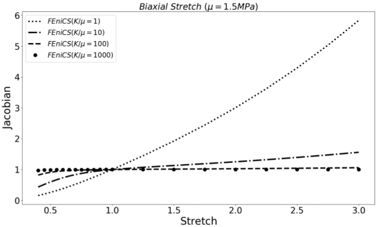
Figure. 5 Effect of compressibility in the Jacobian of deformation gradient tensor in biaxial tension test

It could be seen that by approaching the \(\frac{K}{\mu}\) ratio to 1000, the Jacobian is set to unity regardless of the value of stretch indicating the material is nearly incompressible.

1.4. Compressible Model

1.4.1. Constitutive Equations

The strain energy function for a compressible Neo-Hookean material is defined as:

(42)\[ W=\frac{\lambda}{2}{(lnJ)}^2 + \mu(lnJ) + \frac{1}{2} \mu (I_b-3)\]

In the above equation, the \(\lambda\) is the Lame constant which is equal to \(\frac{E \nu}{(1+\nu)(1-2 \nu)}\) where \(E\) is Young modulus and \(\nu\) is the Poisson ratio. In addition, the stress terms is represented as:

(43)\[ \sigma=J^{-1}[\lambda(lnJ) \textbf{I}+ \mu(\textbf{b}-I)]\]

1.4.2. Finite Element Implementation

A finite element implementation in FEniCS for a biaxial tension test on a unit cube is presented as follows:

from dolfin import *

stretch = [1,1.2,1.4,1.6,1.8,2,2.2,2.4,2.6,2.8,3,3.2,3.4,3.6,3.8,4,4.2,4.4,4.6,4.8,5,5.2,5.4,5.6,5.8,6]

BC = []
for x in range(len(stretch)):
              M = stretch[x] - 1.0
              BC.append(M)

strain = []
print (BC)
for z in range(len(stretch)):
              N = (BC[z])*100
              strain.append(N)


n = 1  # divisions in r direction
mesh = BoxMesh(Point(0, 0, 0), Point(1, 1, 1), n, n, n)

tol = 1E-14
# Define boundaries
def LEFT(x, on_boundary):
              return on_boundary and x[0] < tol

def RIGHT(x, on_boundary):
              return on_boundary and abs(x[0] - 1.0) < tol

def BOTTOM(x, on_boundary):
              return on_boundary and x[1] < tol

def TOP(x, on_boundary):
              return on_boundary and abs(x[1] - 1.0) < tol

def FRONT(x, on_boundary):
              return on_boundary and abs(x[2] - 1.0) < tol

def BACK(x, on_boundary):
              return on_boundary and (x[2]) < tol

boundaries = MeshFunction('size_t', mesh, mesh.topology().dim()-1)
domains = MeshFunction('size_t', mesh, mesh.topology().dim())

ds = Measure("ds", subdomain_data=boundaries)
dx = Measure('dx',subdomain_data=domains)

n = FacetNormal(mesh)

V = VectorFunctionSpace(mesh, 'CG', degree=2)

# Define functions
du  = TrialFunction(V)           # Trial function
v  = TestFunction(V)             # Test function
u  = Function(V)                 # Displacement field

# Kinematics
d = u.geometric_dimension()
I = Identity(d)             # Identity tensor
F = I + grad(u)             # Deformation gradient
C = F.T*F                   # Right Cauchy-Green tensor
b = F * F.T                 # Left Cauchy-Green tensor
Ic = tr(C)
J  = det(F)


nu =0.4
G = 3.5e6
E = 2.*G*(1.+ nu)
mu  = Constant(E/(2*(1 + nu)))
lmbda= Constant(E*nu/((1 + nu)*(1 - 2*nu)))

# Total potential energy
psi = ((lmbda / 2.)*pow(ln(J),2)-mu*ln(J)+0.5*mu*(Ic-3))*dx
F1 = derivative(psi, u, v)

# Compute Jacobian of F
Jac = derivative(F1, u, du)

sigma_11 = []
sigma_22 = []
JJJ = []

def border(x, on_boundary):
              return on_boundary

bound_x =  Expression(("t*x[0]"), degree=1, t=0)
bound_y =  Expression(("t*x[1]"), degree=1, t=0)

SIG = []

for t in range(len(stretch)):

              bound_x.t = BC[t]
              bound_y.t = BC[t]

              bc_x = DirichletBC(V.sub(0), bound_x, border)
              bc_y = DirichletBC(V.sub(1), bound_y, border)
              bc_front = DirichletBC(V.sub(2), Constant((0)), FRONT)
              bc_back = DirichletBC(V.sub(2), Constant((0)), BACK)

              bc_all = [bc_x,bc_y,bc_front]

              problem = NonlinearVariationalProblem(F1, u, bc_all, Jac)

              solver = NonlinearVariationalSolver(problem)
              solver.solve()

              sigma = inv(J) * (lmbda * ln(J) * I + mu * (b - I))
              cauchy = project(sigma, TensorFunctionSpace(mesh, 'DG', 0))

              SIG.append(cauchy(1, 1, 0)[0])

print (SIG)

The obtained result for three different shear modulus (i.e. \(\mu\)) are compared in figure 10:

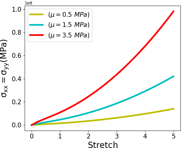
Figure. 6 Stress results of Neo-Hookean compressible model for a single element under biaxial stretch

Note

There is another form of strain energy function for a compressible neo-Hookean material:

(44)\[ W=\frac{1}{2}K(lnJ)^2 + \frac{1}{2} \mu (J^{\frac{-2}{3}} I_b-3)\]

The stress tensor is defined as following:

(45)\[ \sigma=J^{-1}[K \ ln(J)+ \mu J^{\frac{-2}{3}}(\textbf{b}-\frac{1}{3}tr(b) \textbf{I})]\]

In the above equation, \(K\) is the bulk modulus. As a practice you can implement th above equations in the code and compare your results with the previous forms of strain energy function and stress!

1.5. Axisymmetric Model

We consider a sphere which is under an external pressure that could be taken as an axisymmetric problem. This geometry could be seen as revolution of a cross section with respect to the axis of symmetry.

1.5.1. Constitutive Equation

For an axisymmetric problem, the displacement field is defined as following:

(46)\[ u = u_r e_r + u_z e_z\]

The strain energy function is defined as presented in Equation.39. In case of axisymmetric the gradient of displacement field is defined as below:

(47)\[\begin{split} \nabla u = \begin{bmatrix} \frac {\partial u_r}{\partial r} & 0 & \frac {\partial u_r}{\partial z}\\0 & \frac {u_r}{r} & 0\\ \frac {\partial u_z}{\partial r} & 0 & \frac {\partial u_z}{\partial z}\end{bmatrix}\end{split}\]

In general, in case of nonlinear problems, the abstract formulation for nonlinear form is defined as:

(48)\[ F(u,v)=0 \ \forall v \in V\]

In order to find the F in the above equation, first we need to define total potential energy with regard to axisymmetric formulation:

(49)\[ \phi= \int_{V} W(u) \,dV - \int_{\partial V} P \,dA\]

Where \(W\) is the strain energy function and \(P\) corresponds to the loads applied on the boundaries. In the above equation \(dV\) and \(dA\) are the integration symbols over the domains \(V\) and boundaries \(\partial V\). In axisymmetric formulation, we should replace the integration measure \(dV\) and \(dA\) by \(rd \theta dA\) and \(rd \theta ds\) respectively. After substitution in the above equation, the term \(d\theta\) is canceled out from both sides and the above equation yields to:

(50)\[ \phi= \int_{A} W(u) \,rdA - \int_{\partial A} P \,rds\]

In the next step by taking directional derivative from the \(\phi\) with respect to the test function \(v\) , we can find the \(F(u,v)\) as following:

(51)\[ F(u,v)= \lim_{\epsilon\to\infty} \frac {d}{d \epsilon} \phi(u+ \epsilon v)\]

1.5.2. Finite Element Implementation

In order to generate the mesh, we considered the cross section of the sphere as a 2D axisymmetric problem. GMSH was used for mesh generation and structured mesh was created with triangular elements. The red arrows correspond to the external pressure on the sphere. The left edge (e.g., axis of symmetry) is constrained to move in the x direction while the bottom edge is constrained to move in the y direction. The parameters used for this simulation are: \(\mu = 1 MPa\) , \(K = 1 GPa\) and \(P = 10 Pa\) .The dimensions of the geometry, mesh, pressure load and boundary conditions are shown in next figure:

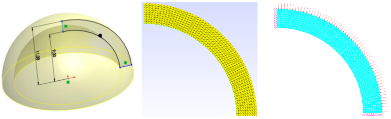
Figure. 7 Geometry of the cross section making the hemisphere (Left), the mesh generated in GMSH (Middle), load and boundary conditions (Right)

The above equations were implemented in FEniCS. The code is presented here:

from dolfin import *

parameters["form_compiler"]["representation"] = "tsfc"

mesh = Mesh("MESH.xml")


facets = MeshFunction("size_t", mesh, "MESH_facet_region.xml")
domains = MeshFunction("size_t", mesh, "MESH_physical_region.xml")

ds = Measure("ds", subdomain_data=facets)
dx = Measure('dx',subdomain_data=domains)

#File("bound.pvd") << facets

x = SpatialCoordinate(mesh)

def GRAD(v):

         return as_tensor([[v[0].dx(0), 0, v[0].dx(1)],
                             [0, v[0]/x[0], 0],
                             [v[1].dx(0), 0, v[1].dx(1)]])


n = FacetNormal(mesh)
p = Constant(100.)


V = VectorFunctionSpace(mesh, 'CG', degree=2)
# Define functions
du  = TrialFunction(V)           # Trial function
v = TestFunction(V)             # Test function
u  = Function(V)                 # Displacement field


d = u.geometric_dimension()
I = Identity(3)
F = I + GRAD(u)             # Deformation gradient

#F = FF(u)

C = F.T*F
b = F*F.T
Ic = tr(C)
J  = det(F)
Ib = tr(b)

Ic_bar = pow(J,-2./3.)*Ic
C_bar = pow(J,-2./3.)*C
B_bar = pow(J,-2./3.)*b

mu = 1E6
K = 1E9


psi = (mu/2. * (Ic_bar - 3.) + 0.5 * K * pow(ln(J),2)) * x[0]*dx - inner(-p*n, u)*x[0]*ds(4)

bcs = [DirichletBC(V.sub(1), Constant(0), facets, 2),
            DirichletBC(V.sub(0), Constant(0), facets, 1)]

F1 = derivative(psi, u, v)

# Compute Jacobian of F
Jac = derivative(F1, u, du)

problem = NonlinearVariationalProblem(F1, u, bcs, Jac)

solver = NonlinearVariationalSolver(problem)


solver.parameters["newton_solver"]["relative_tolerance"]=5e-9

solver.solve()
File("Displacement.pvd") << u

SIGMA_XX = (K * ln(J) / J) * I[0, 0] + (2. / J) * (mu/2. * (B_bar[0, 0] - (1. / 3.) * Ic_bar * I[0, 0]))

SIGMA_YY = (K * ln(J) / J) * I[1, 1] + (2. / J) * (mu/2. * (B_bar[2, 2] - (1. / 3.) * Ic_bar * I[1, 1]))

W = FunctionSpace(mesh, 'P', 1)

STRESS_XX = project(SIGMA_XX, W)
STRESS_YY = project(SIGMA_YY, W)

File("SIG_X.pvd") << STRESS_XX
File("SIG_Y.pvd") << STRESS_YY

The same model with the same geometry, loading, boundary conditions and mesh was generated in ANSYS APDL.

The PLANE 182 element was used for the simulation in ANSYS with axisymmetric element behavior. The displacement results in the x and y directions obtained from ANSYS and FEniCS implementation are shown in the figures:

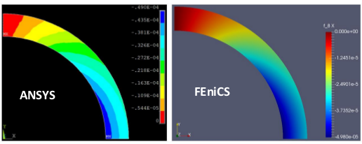
Figure. 8 The displacement results in X direction (FEniCS) vs ANSYS

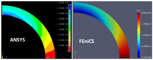
Figure. 9 The displacement results in Y direction (FEniCS) vs ANSYS

1.6 von-Mises Fiber Model

Note

Please read this paper and this paper for more details about this model.

1.6.1. Introduction

The strain energy function is defined as following:

(52)\[ W = W_{matrix}+W_{fiber}\]

The ground substance \(W_{matrix}\) is defined as Neo-Hookean material with this energy function:

(53)\[ W_{matrix} = c_{1}(I_1-3)\]

The part of strain energy function which is related to the fibers is presented as:

(54)\[ W_{matrix} = \int_{\theta_p- \frac{\pi}{2}}^{\theta_p + \frac{\pi}{2}} P(\theta) W_{fiber} \circ I_4 (\theta) d \theta\]

In the above equation, the fourth invariant of \(C\) tensor \(I_4 (\theta)\) is:

(55)\[ I_4 (\theta) = a_0 (\theta) . C . a_0 (\theta) = \lambda^2 (\theta)\]

Where \(a_0 (\theta)\) defines the orientation of the fibers. In addition, \(P(\theta)\) is the distribution function defined as:

(56)\[ P(\theta) = \frac{1}{\pi I_0 (k)} e^{k \cos (x)} dx\]

\(k\) is the fiber concentration factor and \(\theta_p)\) is the preferred fiber orientation. The strain energy function associated with collagen fibers family is defined as following:

(57)\[ \lambda (\theta) \frac{\partial W_{fiber} \circ I_4 (\theta)}{\partial \lambda(\theta)} = c_3 (e^{c_4 (\lambda (\theta) - 1} -1)\]

Where \(c_3\) is the exponential fiber stress coefficient and \(c_4\) is the rate of uncrimping collagen fibers.

1.6.2. Stress Tensor

The second Piola-Kirchhoff stress tensor could be represented as:

(58)\[ \mathbf{S} = pJ \mathbf{C^{-1}} + 2J^{\frac{-2}{3}} DEV[\frac{\partial W}{\partial C}]\]

Note

The operator \(DEV[.]\) is the deviatoric projection operator.

We start with the matrix part and by using chain rule:

(59)\[ \frac{\partial W}{\partial C} = \frac{\partial W}{\partial I_1} \times \frac{\partial I_1}{\partial C}\]

The second term on the right hand side of the above equation is equal to identity tensor (See Equation.6

On the other hand:

(60)\[ \frac{\partial W_{fiber}}{\partial C} = c_1 \mathbf{I}\]

(61)\[ S = pJC^{-1}+2J^{\frac{-2}{3}} [c_1 I - \frac{1}{3}(c_1 I : C)C^{-1}]\]

We know that \(I:C=I_1\):

(62)\[ S = pJC^{-1}+2J^{\frac{-2}{3}} [c_1 (I - \frac{1}{3} I_1 C^{-1})]\]

We derive the stress term for the fiber part. The strain energy function for the fibers is derived from \(W_{fiber} \circ I_4(\theta)\) :

(63)\[ S = 2J^{\frac{-2}{3}} DEV [\frac{\partial W_{fiber} \circ I_4 (\theta)}{\partial C}]\]

The term in the bracket could be rewritten using the chain rule:

(64)\[ \frac{\partial W_{fiber} \circ I_4 (\theta)}{\partial C} = \frac{\partial W_{fiber} \circ I_4 (\theta)}{\partial I_4} \times \frac{I_4}{\partial C}\]

The first term in the right hand side of the above equation, could be presented again using the chain rule:

(65)\[ \frac{\partial W_{fiber} \circ I_4 (\theta)}{\partial I_4} = \frac{\partial W_{fiber} \circ I_4 (\theta)}{\partial \lambda (\theta)} \times \frac{\partial \lambda (\theta)}{\partial I_4}\]

We know that \(I_4 (\theta)= \lambda^2 (\theta)\) . Thus, the second term in the right hand side of the above equation could be simplified to:

(66)\[ \frac{\partial I_4}{\partial \lambda (\theta)} = 2\lambda (\theta) \Rightarrow \frac{\partial \lambda (\theta)}{\partial I_4} = \frac {1}{2 \lambda (\theta)}\]

We know that:

(67)\[ \lambda (\theta) \frac{\partial W_{fiber} \circ I_4 (\theta)}{\partial \lambda (\theta)} = c_3 [e^{c_4(\lambda(\theta)-1)}-1]\]

Then by combining the equations:

(68)\[ \frac{\partial W_{fiber} \circ I_4 (\theta)}{\partial I_4} = \frac{1}{2 \lambda^2 (\theta)} c_3 [e^{c_4 (\lambda (\theta)-1)}-1] = \eta\]

And then we can write:

(69)\[ S = 2J^{\frac{-2}{3}}[a_0 (\theta).a_0 (\theta) \int_{\theta_p- \frac{\pi}{2}}^{\theta_p + \frac{\pi}{2}} P(\theta) \eta d \theta - [ \frac{1}{3} a_0 (\theta).a_0 (\theta):C \times \int_{\theta_p- \frac{\pi}{2}}^{\theta_p + \frac{\pi}{2}} P(\theta) \eta d \theta ]C^{-1}]\]

(70)\[ S = 2J^{\frac{-2}{3}}[\int_{\theta_p- \frac{\pi}{2}}^{\theta_p + \frac{\pi}{2}} P(\theta) \eta d \theta[a_0 (\theta).a_0 (\theta) - \frac{1}{3} I_4 C^{-1}] d \theta ]\]

Now by combining with the stress obtained from the strain energy of the matrix part:

(71)\[ \mathbf{S} = pJC^{-1} + 2J^{\frac{-2}{3}}[c_1 (I - \frac{1}{3} I_1 C^{-1}) + \int_{\theta_p- \frac{\pi}{2}}^{\theta_p + \frac{\pi}{2}} P(\theta) \eta [a_0 (\theta).a_0 (\theta)-\frac{1}{3} I_4 C^{-1}] d \theta ]\]

The Cauchy stress yields to:

(72)\[ \mathbf{\sigma} = \frac{1}{J} F.S.F^T = P \mathbf{I}+ \frac{2}{J}[c_1(\mathbf{B}-\frac{1}{3}I_1 \mathbf{I}]+\int_{\theta_p- \frac{\pi}{2}}^{\theta_p + \frac{\pi}{2}} P(\theta,k)W_4 I_4 [a_0 (\theta) \otimes a_0 (\theta)-\frac{1}{3} \mathbf{I}] d \theta]\]

Note

The \(\mathbf{B}\) is the left cauchy stress tensor and \(W_4(\theta)= \frac{1}{2 \lambda^2 (\theta)}c_3 [e^{c_4(\lambda (\theta) - 1)}-1]\)

1.6.3. Strain Energy Function

In general the strain energy function in the von-Mises fiber model is represented as:

(73)\[ \tilde{W}= F_m (\tilde{I_1}) + \int_{\theta_p-\frac{\pi}{2}}^ {\theta_p+\frac{\pi}{2}} P(\theta) F(\tilde{\lambda}) d \theta+\frac{K}{2}[Ln(J)]^2\]

Where \(F_m (\tilde{I_1})\) corresponds to the contribution from the matrix:

(74)\[ F_m(\tilde{I_1})=c_1(\tilde{I_1}-3)\]

The contribution from the fiber part is:

(75)\[ F_f(\tilde{\lambda})=c_3(e^{-c_4}[Ei(c_4 \tilde{\lambda})-Ei(c_4)]-Ln(\tilde{\lambda}))\]

The \(\tilde{\lambda}\) is the stretch represented as following:

(76)\[ \tilde{\lambda}^2=\tilde{I}_4= \textbf{a}_0 (\theta).\tilde{\textbf{C}}.\textbf{a}_0(\theta)\]

The distribution function is expressed as:

(77)\[ P(\theta)=\frac{1}{\pi I_0(k_f)}e^{k_f cos2(\theta-\theta_p)}\]

In the above, the \(I_0(k_f)\) is the the Bessel function of the first kind:

(78)\[ I_0 (k_f)=\frac{1}{\pi} \int_{0}^{\pi} e^{k_fcos(x)}dx\]

1.6.4. Finite Element Implementation

We implement this model in a finite element code on a cube element where the fibers are aligned in Y direction (Vertical) and the element is under biaxial stretch. The values of the constants of \(c_1\) , \(c_3\) and \(c_4\) are equal to 10Pa, 50 Pa and 5 respectively. In addition the bulk modulus \(K\) is equal to 1 GPa. We implement the numerical integration by trapezoidal rule. In addition, in order to define the plane where the fibers are confined with, we should use Discontinuous Galerkin function space and then assign the vector values \(\vec{a}\) and \(\vec{b}\) to each element by using the index of the elements. Here is the FEniCS implementation and validation against the analytical solution:

from dolfin import *
import sys
sys.setrecursionlimit(10000)
import numpy as np


stretch = [1.,1.05,1.1,1.15,1.2,1.25,1.3,1.35,1.4,1.45,1.5,1.55,1.6]

BC = []

for x in range(len(stretch)):
    N = stretch[x] - 1.0
    BC.append(N)

tol = 1E-14

# Define boundary
def LEFT(x, on_boundary):
    return on_boundary and x[0] < tol

def RIGHT(x, on_boundary):
    return on_boundary and abs(x[0] - 1.0) < tol

def BOTTOM(x, on_boundary):
    return on_boundary and x[1] < tol

def TOP(x, on_boundary):
    return on_boundary and abs(x[1] - 1.0) < tol

def FRONT(x, on_boundary):
    return on_boundary and abs(x[2] - 1.0) < tol

def BACK(x, on_boundary):
    return on_boundary and (x[2]) < tol


mesh = UnitCubeMesh.create(1,1,1,CellType.Type.tetrahedron)
n = FacetNormal(mesh)

V = VectorFunctionSpace(mesh, 'CG', degree=1)

du  = TrialFunction(V)           # Trial function
v  = TestFunction(V)             # Test function
u  = Function(V)
#############################################

boundaries = MeshFunction('size_t', mesh, mesh.topology().dim()-1)
subdomains = MeshFunction('size_t', mesh, mesh.topology().dim())


dx = Measure('dx', domain=mesh, subdomain_data=subdomains, metadata={'quadrature_degree': 10})


d = u.geometric_dimension()
I = Identity(d)             # Identity tensor
F = I + grad(u)             # Deformation gradient
C = F.T*F
b = F*F.T
Ic = tr(C)
J  = det(F)
Ib = tr(b)

Ic_bar = pow(J,-2./3.)*Ic
C_bar = pow(J,-2./3.)*C
B_bar = pow(J,-2./3.)*b


def trapezoidal(f, a, b, n):

    h = float(b - a) / n
    s = 0.0
    s += f(a)/2.0
    for i in range(1, n):
        s += f(a + i*h)
    s += f(b)/2.0
    return s * h

c_1 = 10.
c_3 = 50.
c_4 = 5.
gamma = 0.5772156649

# The fiber concentration factor
K=0.

# The bulk modulus
KK =  1E6



def bessel(x):

    return (1. / (np.pi)) * np.exp(K * np.cos(x))

          .
          .
          .

######### Theta_p : Fiber preferred orientation  #########

#theta_p =  0           # Tangential orientation
theta_p = np.pi / 2.  # Meridional orientation
#theta_p = np.pi / 4.

######### This function returns:  P(theta) * F_2(lambda)  #########

def stress_integral(theta):
    a_vector = as_vector([cos(theta) * a1, cos(theta) * a2, cos(theta) * a3])
    b_vector = as_vector([sin(theta) * b1, sin(theta) * b2, sin(theta) * b3])
                        .
                        .
                        .
                        .


sigma_11 = []
sigma_22 = []
JJJ = []


for i in range(len(BC)):
                .
                .
                .
                .


print(sigma_11)
print(sigma_22)

Here is the results and comparison with the analytical solution:

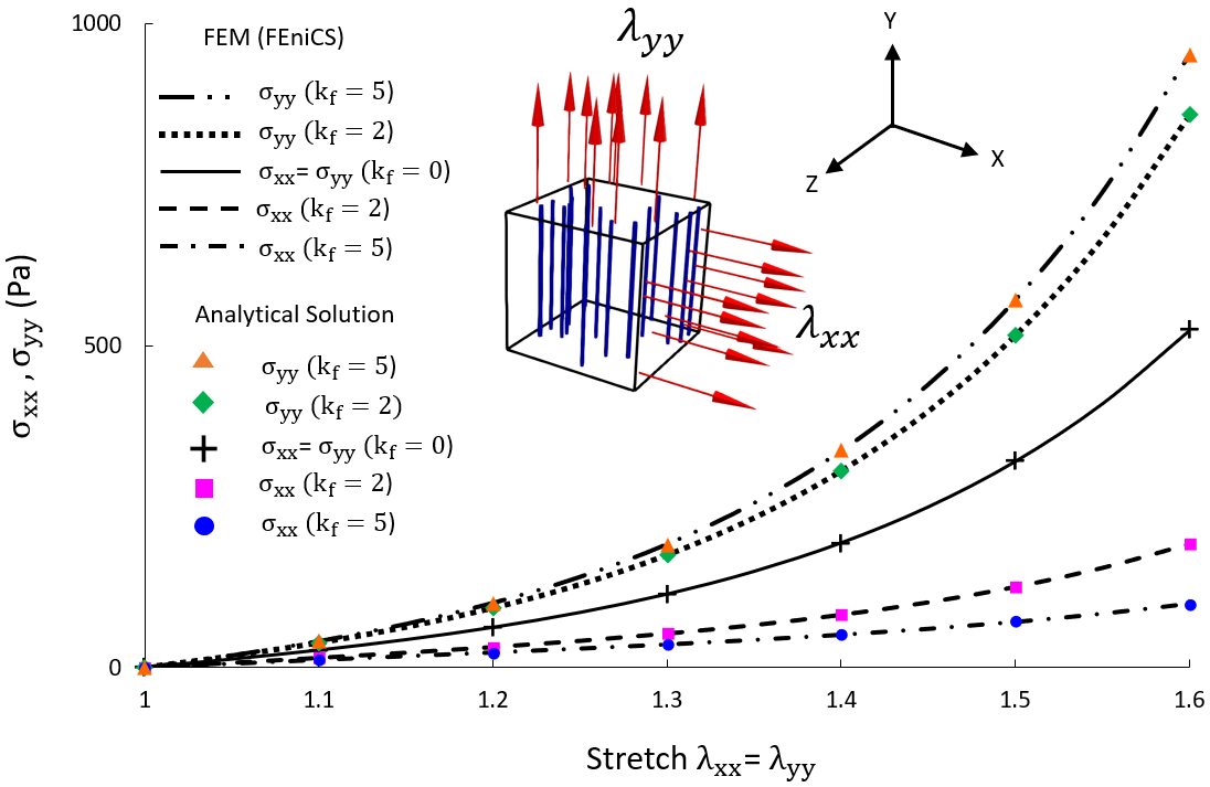
Figure. 10 Stress results of the von-Mises fiber model when a unit cube is under biaxial stretch in comparison with the analytical solution

Note

The complete FEniCS code is available upon request (Please refer to the section : About the Author)