3. Drug Delivery Simulation
3.1 Iontophoresis
Iontophoresis is a noninvasive delivery system designed to overcome barriers to ocular penetration of topical ophthalmic medications by employing a low-amplitude electrical current to promote the migration of a charged drug substance across biological membranes. This method is used for enhancing the drug delivery into the biological tissues. In general, an increase in the electric current density and the duration of the application enhances drug penetration. Despite the increase in drug permeation achieved with increased electric current density and time, importantly, it must be remembered that the safety of ocular iontophoresis is correlated with these parameters. Iontophoresis is a non-invasive method of transferring ionized drugs through membranes with low electrical current. The drugs are moved across the membranes by two mechanisms including migration and electro-osmosis.
The most important eye diseases related to the posterior of the eye includes glaucoma. Drug penetration into the eye may be increased with iontophoresis, the process of moving a charged molecule by an electric current across the cornea or sclera. Transcorneal iontophoresis has been shown to result in significantly higher drug levels than those found after multiple drop treatments. The properties of the sclera (hydration, leakiness, low electrical resistance) make the iontophoretic delivery feasible at low electric currents or voltages. The important parameters determining the drug’s penetration are: Intensity of the electric field, drug concentration and duration of the iontophoresis procedure. A good review about
Ocular iontophoresis
This is the process of delivery of the drug to a particular area of the eye as shown in this figure:
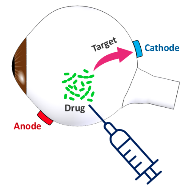
Figure. 13 Illustration of OCULAR iontophoresis. The target is the sclera at the posterior of the eye globe
The drug which is usually positively charged particles are injected into the eye globe. The electrodes should be attached at appropriate locations to the eye globe. The sclera tissue itself contains negative charges due to existence of glycosaminoglycans (GAGs). After injection of the drug, some of the injected drug penetrates inside the sclera by free diffusion in order to maintain the electro-neutrality condition. However, it is always desirable to enhance the penetration of the drug into the tissue. This could be done by applying an external electrical voltage.
3.2 Simulation using FEM
The numerical simulation of the iontophoresis is based on solving the PNP system as described in chapter 2. The computational domain is presented as a simplified 2D geometry of the eye globe. The main sub-domains including sclera, aqueous humor and cornea are shown in this figure:
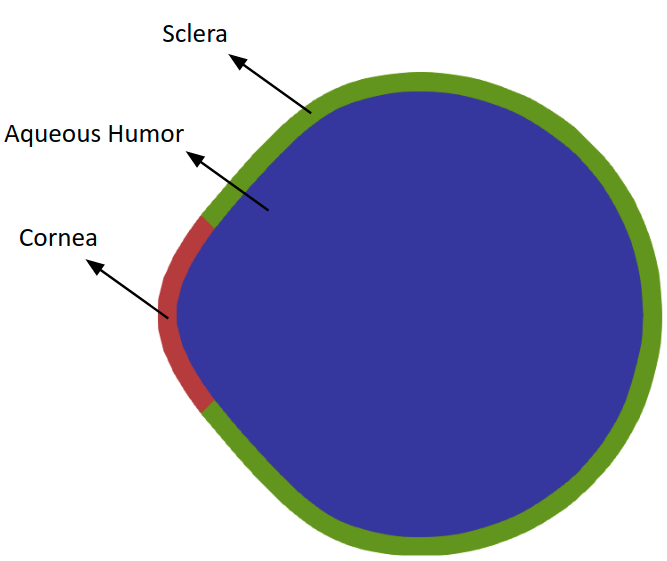
Figure. 14 The 2D geometry of the eye globe used in the simulation of drug delivery to the posterior of the eye globe
For the simplicity, the sclera and the cornea are considered as a single subdomain.
In this simulation, it is assumed that the drug has been injected into the eye inside the aqueous humor. The location of the electrodes and the target where the enhancement of drug delivery is desired were illustrated in the Figure 19. It should be noted that, the drug consist of positively charged particles. After injection of the drug, it diffuses inside the sclera because of the fact that the sclera tissue contain fixed negative charges stemming from glycosaminoglycans (GAGs) which are negatively charged chemical groups. After application of the drug, in order to maintain the electroneutrality, a part of the injected drug freely diffuses inside the sclera. However, the purpose of the iontophoresis is to increase the concentration of the drug inside a specific target. For example in this example, the target is an area at the posterior of the eye globe. After application of the voltage to the electrodes, the diffusion of the drug increases in time at the target zone. It should be noted that aside from the positively charged drug particles, there exists some negatively charged ions inside the eye (e.g., Chloride anions). In this simulation we assume the concentration of the positively charged drug and the negatively charged anions is equal to 10 mM while the concentration of the fixed charges attached to the sclera tissue is 5 mM. The process of the iontophoresis is done under application of 2V for nearly 4 minutes.
The FEniCS code for this simulation is presented here:
from dolfin import *
import numpy as np
from sympy import Heaviside
import math


#Diffusion constant for Drug+ cations GEL
D_Drug = 1.16 * (10**(-6.))

#Diffusion constant for Cl- anioins GEL
D_negative_charges = 1.6 * (10**(-9.))

#Diffusion constant for Drug+ cations SOLUTION
D_Drug_s = 1.16 * (10**(-9.))

#Diffusion constant for Cl- anioins SOLUTION
D_negative_charges_s = 1.6 * (10**(-9.))

#The gas constant
R = 8.31

#Initial value for Drug+ in the solution
c_init_Drug_aqueous_humor = 10

#Initial value for Cl- in the solution
c_init_negative_charges_aqueous_humor = 10


#Initial value for fixed anioin (e.g. bound charge) in the sclera
c_init_Fixed_sclera = 5


#The initial concentration of the drug and negative charges inside the sclera
c_init_Drug_sclera = ((c_init_Fixed_sclera+pow(c_init_Fixed_sclera**2+4*pow(c_init_Drug_aqueous_humor,2),0.5)))/2.
c_init_negative_charges_sclera = ((-c_init_Fixed_sclera+pow(c_init_Fixed_sclera**2+4*pow(c_init_negative_charges_aqueous_humor,2),0.5)))/2.

##############################
#Valence of Drug+
z_Drug = 1.0

#Valence of negative charges
z_negative_charges = -1.0

#Valence of Fixed charges
z_Fixed = -1.0


eps_vacume = 8.85*pow(10,-12)
eps_water = 80.
eps_sclera = 67.

#Dielectric permittivity
epsilon = eps_vacume * eps_water
epsilon_p = eps_vacume * eps_sclera


#Temperature
Temp = 293.0

#Electrical mobility for Drug+ cations
mu_Drug = D_Drug / (R*Temp)
#Electrical mobility for charged ions
mu_negative_charges = D_negative_charges / (R*Temp)


#Faraday number
Faraday = 96483.34

#Reading the mesh
mesh = Mesh()
hdf = HDF5File(mesh.mpi_comm(), "0file.h5", "r")
hdf.read(mesh, "/mesh", False)
subdomains = MeshFunction('size_t', mesh, mesh.topology().dim())


hdf.read(subdomains, "/subdomains")
boundaries = MeshFunction('size_t', mesh, mesh.topology().dim()-1)
hdf.read(boundaries, "/boundaries")


dx = Measure('dx', domain=mesh, subdomain_data=subdomains)

#Defining element for scalar variables (e.g. concentrations and voltage)
Element1 = FiniteElement("CG", mesh.ufl_cell(), 1)

# Defining the mixed function space
W_elem = MixedElement([Element1, Element1 ,Element1])

W = FunctionSpace(mesh, W_elem)

#Defining the "Trial" functions
z = Function(W)
dz=TrialFunction(W)

#separating the unknown variables
c_Drug, c_negative_charges,  phi = split(z)

#Defining the "test" functions
(v_1, v_2,v_6) = TestFunctions(W)

# Time variables
dt = 1
t = 0
T = 247

#Required function spaces
V_c_Drug = FunctionSpace(mesh, Element1)
V_c_negative_charges = FunctionSpace(mesh, Element1)
V_phi = FunctionSpace(mesh, Element1)

#MeshFunction is defined to be used later for distinguishing between the sclera domain and aqueous humor domain
materials = MeshFunction("size_t", mesh, mesh.topology().dim())

#The index of the elements corresonding to the sclera domain should be extracted from the mesh file and given here
gel_ind = [0, 1, 2, 3, 4, 5, 6, 7, 8, 9, 10, 11, ....]

# Defining the initial conditions for the drug
class Drug_initial(UserExpression):

         def __init__(self, **kwargs):
                  super().__init__()


                  self.c_Drug_sclera = kwargs["c_Drug_sclera"]
                  self.c_Drug_aqueous_humor = kwargs["c_Drug_aqueous_humor"]
                  self.materials = kwargs["materials"]

         def eval_cell(self, value, x, cell):

                  if self.materials[cell.index] in gel_ind:
                      value[0] = self.c_Drug_sclera

                  else:
                      value[0] = self.c_Drug_aqueous_humor

         def value_shape(self):
                  return ()

IC_Drug = Drug_initial(materials=materials,c_Drug_sclera = c_init_Drug_sclera, c_Drug_aqueous_humor = c_init_Drug_aqueous_humor, degree=0)

# Previous solution
C_previous_Drug = interpolate(IC_Drug, V_c_Drug)

# Defining the initial conditions for the negative charges
class negative_charges_initial(UserExpression):

         def __init__(self, **kwargs):

                  super().__init__()
                  self.c_negative_charges_sclera = kwargs["c_negative_charges_sclera"]
                  self.c_negative_charges_aqueous_humor = kwargs["c_negative_charges_aqueous_humor"]
                  self.materials = kwargs["materials"]


         def eval_cell(self, value, x, cell):

                  if self.materials[cell.index] in gel_ind:
                      value[0] = self.c_negative_charges_sclera

                  else:
                      value[0] = self.c_negative_charges_aqueous_humor

         def value_shape(self):
                  return ()

IC_negative_charges = negative_charges_initial(materials=materials,c_negative_charges_sclera = c_init_negative_charges_sclera, c_negative_charges_aqueous_humor = c_init_negative_charges_aqueous_humor, degree=0)

# Previous solution
C_previous_negative_charges = interpolate(IC_negative_charges, V_c_negative_charges)


#VaritioDrugl form for the Nernst-Planck equation in the sclera domain for Drug+ and negative charges
#Note that 33 and 34 correspond to the sclera domain and aqueous humor domain
Weak_NP_Drug = c_Drug * v_1 * dx(33) + dt * D_Drug * dot(grad(c_Drug), grad(v_1)) * dx(33) +\
                             dt * z_Drug * mu_Drug * Faraday * c_Drug * dot(grad(phi), grad(v_1)) * dx(33) - C_previous_Drug * v_1 * dx(33)

Weak_NP_negative_charges = c_negative_charges * v_2 * dx(33) + dt * D_negative_charges * dot(grad(c_negative_charges), grad(v_2)) * dx(33) +\
                             dt * z_negative_charges * mu_negative_charges * Faraday * c_negative_charges * dot(grad(phi), grad(v_2)) * dx(33) - C_previous_negative_charges * v_2 * dx(33)


#VaritioDrugl form for the Poisson equation in the sclera domain for Drug+ and Cl- and fixed charge
Weak_Poisson = dot(grad(phi), grad(v_6)) * dx(33) - (Faraday / epsilon_p) * z_Drug * c_Drug * v_6 * dx(33) \
                                     - (Faraday / epsilon_p) * z_negative_charges * c_negative_charges * v_6 * dx(33)- (Faraday / epsilon_p) * z_Fixed * c_init_Fixed_sclera * v_6 * dx(33)

##################################

#VaritioDrugl form for the Nernst-Planck equation in the aqueous humor domain for Drug+ and negative charges
Weak_NP_Drug_aqueous_humor = c_Drug * v_1 * dx(34) + dt * D_Drug_s * dot(grad(c_Drug), grad(v_1)) * dx(34) +\
                             dt * z_Drug * mu_Drug * Faraday * c_Drug * dot(grad(phi), grad(v_1)) * dx(34) - C_previous_Drug * v_1 * dx(34)

Weak_NP_negative_charges_aqueous_humor = c_negative_charges * v_2 * dx(34) + dt * D_negative_charges_s * dot(grad(c_negative_charges), grad(v_2)) * dx(34) +\
                             dt * z_negative_charges * mu_negative_charges * Faraday * c_negative_charges * dot(grad(phi), grad(v_2)) * dx(34) - C_previous_negative_charges * v_2 * dx(34)


#VaritioDrugl form for the Poisson equation in the aqueous humor domain for Drug+ and negative charges and fixed charge
Weak_Poisson_aqueous_humor = dot(grad(phi), grad(v_6)) * dx(34) - (Faraday / epsilon) * z_Drug * c_Drug * v_6 * dx(34) \
                                     - (Faraday / epsilon) * z_negative_charges * c_negative_charges * v_6 * dx(34)


#Summing up variatioDrugl forms
F = Weak_NP_Drug + Weak_NP_negative_charges + Weak_Poisson + Weak_NP_negative_charges_aqueous_humor + Weak_NP_Drug_aqueous_humor + Weak_Poisson_aqueous_humor

#Defining the boundary conditions
#Note that 35 and 36 correspond to the boundaries where the anode and cathode have been placed on
#W.sub(0)  and W.sub(1) refer to the concentration of the drug and tthe negative charges respectively
bc_left_c = DirichletBC(W.sub(0),Constant(c_init_Drug_sclera), boundaries, 35)
bc_right_c = DirichletBC(W.sub(0),Constant(c_init_Drug_sclera), boundaries, 36)

bc_left_c_1 = DirichletBC(W.sub(1),Constant(c_init_negative_charges_sclera), boundaries, 35)
bc_right_c_1 = DirichletBC(W.sub(1),Constant(c_init_negative_charges_sclera), boundaries, 36)

#Saving the results for the concentration of the drug
q = File("Drug.pvd")


assign(z.sub(1), C_previous_negative_charges)
assign(z.sub(0), C_previous_Drug)

#Solving block
#W.sub(2) refers to the voltage

while t <= T:

         bc_left_volt = DirichletBC(W.sub(2), -1 * Heaviside((t - 37), 0), boundaries, 35)
         bc_right_volt = DirichletBC(W.sub(2), 1 * Heaviside((t - 37), 0), boundaries, 36)
         bcs = [bc_left_volt, bc_right_volt, bc_left_c, bc_right_c, bc_left_c_1, bc_right_c_1 ]

         J = derivative(F, z, dz)

         problem = NonlinearVariatioDruglProblem(F, z, bcs, J)
         solver = NonlinearVariatioDruglSolver(problem)
         solver.parameters['newton_aqueous_humorver']['convergence_criterion'] = 'incremental'
         solver.parameters['newton_aqueous_humorver']['linear_aqueous_humorver'] = 'mumps'
         solver.solve()

         (c_Drug, c_negative_charges,phi) = z.split(True)

         C_previous_Drug.assign(c_Drug)
         C_previous_negative_charges.assign(c_negative_charges)

################################################
         t += dt
         q << c_Drug
Finally the video of this simulation is presented here which is 6X faster. It could be clearly seen how diffusion of the drug increases with time at the posterior of the globe due to application of the electrical field.
Note
The geometry was created based on almost real dimensions of the eye globe and the mesh was generated in GMSH. The mesh file and the FEniCS code are available inside the repository in the folder: Drug Delivery